4a. Measurement architecture

NoteWhere am I in the pipeline?

• Inputs: The harmonised item map at outputs/item_mapping_overview.csv; the pooled retained-item keys at outputs/tables/first_order_pooled_optimized_map_s2_s3_s5.csv and outputs/tables/higher_order_pooled_optimized_map_s2_s3_s5.csv; the wrangled item-level parquet files in data/wrangled_data/ for S1–S5; and four dedicated cross-study measurement repositories owned by this page and cached under outputs/measurement_models/. The first-order layer comprises the stand-alone one-factor CFA repository (first_order/fo_<study>_<construct>_all.rds), the pooled S2/S3/S5 multigroup refinement repository (pooled_refinement/pooled_<construct>_*_*.rds), and the joint correlated-factor CFA repository (first_order_joint/fo_joint_<study>_all.rds). The higher-order layer reuses the same parquet item files via the higher-order, pooled-higher-order, and joint-higher-order repositories (higher_order/, higher_order_pooled/, higher_order_joint/). A representation-comparison repository (representation_comparison/repcomp_<study>_<item-key>_<family>.rds) feeds the four-family system-level comparison.
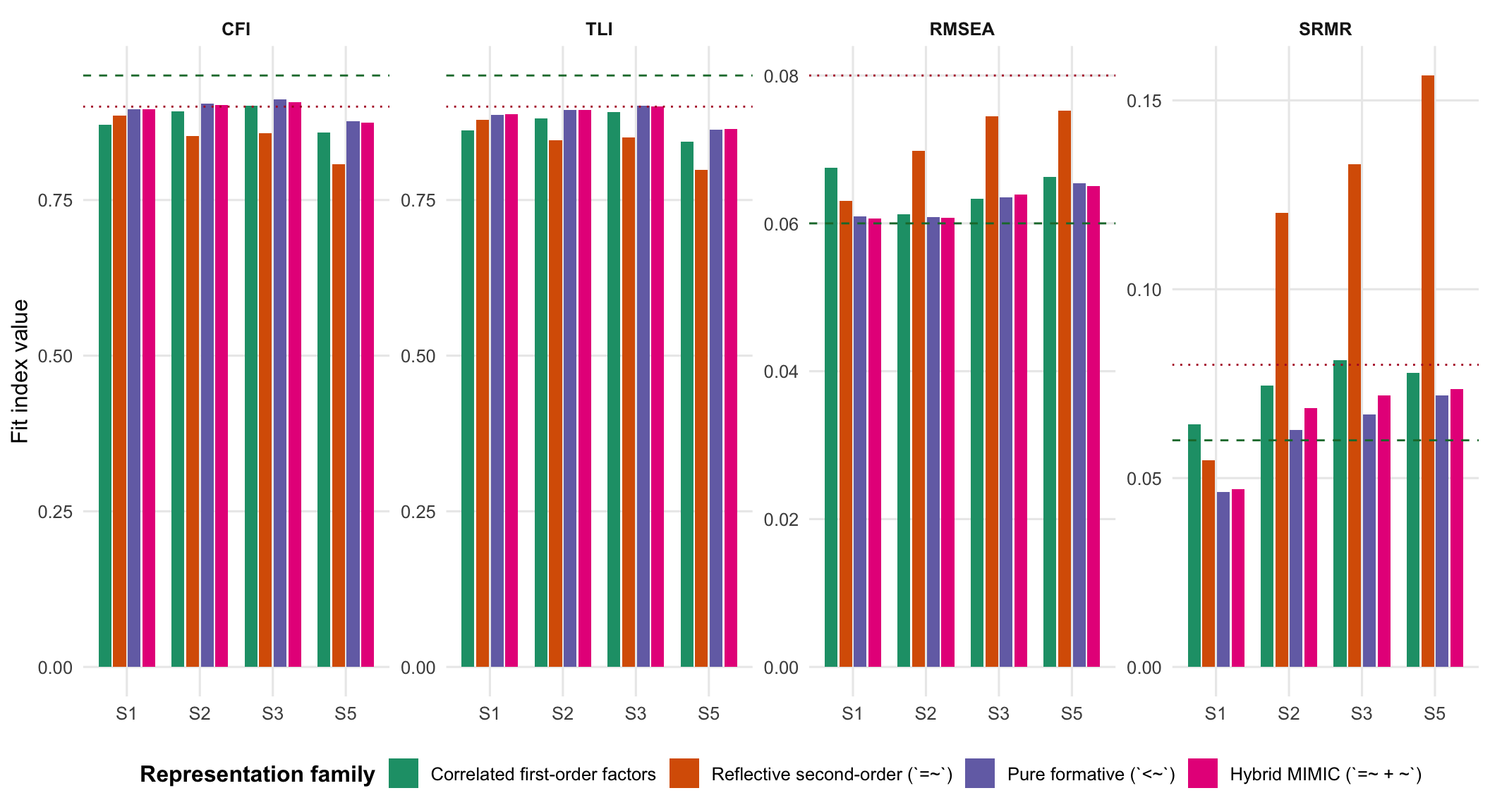
• This page: Measurement architecture (Stages 2 and 3). Synthesises first-order measurement validation and higher-order construct modelling across waves: cross-study loading stability, reliability per construct per wave, and joint discriminant-validity diagnostics now all source from the harmonised first-order CFA repositories. The second-order section adds a mapping-driven four-family representation comparison (correlated first-order, reflective second-order =~, pure formative <~, hybrid MIMIC =~ + ~) estimated twice: once with all available mapped items and once with the pooled optimized retained item IDs.
• Hands off to: 4b FIMI DV operationalisation (Stage 4 — criterion derivation) · 4c FIMI prediction (Stage 5 — structural prediction) · 4d Deployment and invariance (Stages 6 + 7 — scale reduction and multi-group invariance) · 4e Nomological network (Stage 8 — external validity).

Overview

What this page establishes. First-order construct blocks replicate across waves wherever the same items are re-administered: loadings, ω, and AVE sit in a comparable band across S1–S5. The five higher-order composites (THREAT, ABAND, FEAR, SUPF, GEN) are defensible but not strictly unidimensional — the one-factor reflective form is the wrong null, and the diagnostics in this section operate as flags for review rather than pass/fail gates. Discriminant validity has theory-consistent caveats: the highest HTMT / lowest sqrt(AVE) margins concentrate exactly where the substantive theory predicts content overlap (abandonment first-order trio; THREAT–ABAND at the composite level). At the representation layer, the comparison is now mapping-driven and item-key-sensitive, with the best-performing item key reported in the main text and the alternate key retained as a collapsed sensitivity check.

This page synthesises the measurement half of the DisInformeter pipeline: Stage 2 (first-order construct validation) and Stage 3 (higher-order construct modelling). It is the cross-study companion to the per-wave estimation pages 3a–3e and answers three questions that no per-wave page can answer on its own:

1. Do the first-order construct blocks behave the same way across waves and samples? We compare standardised indicator loadings, single-factor reliability (α, ω), and AVE for every first-order construct that recurs across S1, S2, S3, and S5, working from the harmonised item map rather than inheriting wave-specific composite-layer choices. S4 is structurally absent from this layer: the deployment instrument fields direct higher-order composite indicators rather than first-order parent blocks, so first-order diagnostics are undefined on the S4 indicator set.
2. What happens when first-order validation is rebuilt directly from the item map rather than inherited from the full SEMs? We fit a stand-alone one-factor CFA repository (one model per construct × wave), a joint correlated-factor CFA repository (one model per wave with every first-order construct as a correlated reflective factor), and a pooled S2/S3/S5 multigroup refinement repository, all driven by outputs/item_mapping_overview.csv. The cross-wave loading-stability, reliability, HTMT, and Fornell–Larcker sections now read directly from these repositories — they no longer inherit the legacy per-study SEM fits.
3. Which higher-order representation wins, where, and at what cost? We compare the three construct-representation families — fully reflective (=~), pure formative composite (<~), and hybrid MIMIC (=~ + ~) — across the studies that fielded them.

All four measurement repositories are owned here and cached under outputs/measurement_models/. Rerenders reuse the same cache, and the construct × wave fits are parallelised over (study × construct) and (study × family) jobs via future::multisession (DISINFORMETER_SEM_WORKERS, default on this page: 12). FIMI criterion derivation (Stage 4), cross-study FIMI prediction (Stage 5), invariance ladders (Stage 7), and external-validity evidence (Stage 8) live on 4b, 4c, 4d, and 4e, respectively.

Operator legend

In lavaan syntax, =~ defines reflective measurement (a latent factor’s indicators are caused by the factor); <~ defines a pure formative composite (the composite is a weighted aggregate of its components and has no reflective indicators); and ~ is a regression between observed or latent variables. The hybrid MIMIC representations used on this page combine the first two: a higher-order latent is reflectively identified by direct affective indicators via =~ and simultaneously regressed on its first-order parents via ~. The pure formative variants drop the =~ indicators and identify the composite from its first-order parents alone via <~.

Table 1: lavaan operator legend used throughout the cross-study pages.

Operator	Meaning	Example
`=~`	Reflective measurement: indicators are caused by the latent.	`THREAT =~ th9 + th4 + th6`
`<~`	Pure formative composite: the composite is a weighted aggregate of its components; no reflective indicators.	`THREAT <~ EXPL + GAY + MIGR`
`~`	Structural regression between (latent or observed) variables.	`FIMI ~ THREAT + ABAND + FEAR + SUPF`

The hybrid MIMIC notation =~ + ~ is shorthand for the simultaneous combination of the two operators on the same higher-order latent — it is not a separate lavaan operator. The other cross-study pages reference this legend rather than repeat the prose.

Cross-study first-order measurement

Stage 2 asks whether each first-order construct block survives outside its original sample. This section is now sourced end-to-end from a harmonised first-order measurement repository owned by this page — the legacy synthesis that pulled standardised loadings, reliability, and discriminant-validity inputs out of the per-study full SEM fits has been retired. The legacy fits mixed three different identifying conventions (S1’s borrowed-indicator hybrid plus a two-step rescue, S2 / S3’s hybrid MIMIC plus anchored formative, S5’s measurement-only hybrid) and inherited residual choices that pre-dated the harmonised item map, so the cross-wave numbers they produced for first-order constructs were not strictly comparable. The repository below removes that inconsistency by re-estimating every first-order CFA against the same item set and the same MLR / FIML routine.

Model repository from the item map

The repository is the source of truth for Stage-2 first-order validation. It does the following in one reproducible, parallelisable pass:

• reads the mapped first-order items in outputs/item_mapping_overview.csv;
• resolves legacy names (lgbt* → lgb*, prag_kin* → pkin*, pch* ←→ pkin*) against the wrangled item files;
• fits one stand-alone one-factor CFA per construct × wave for S1, S2, S3, and S5 — the source of single-factor reliability (α, ω), AVE, and per-cell loading diagnostics;
• fits one joint correlated-factor CFA per wave (S1, S2, S3, S5) with every first-order construct entering as a correlated reflective factor — the source of Φ (latent correlations) and joint-fit standardised loadings used in HTMT / Fornell–Larcker;
• fits a pooled S2/S3/S5 refinement repository on item identity columns, so Lithuanian, German, and S5 aliases of the same item are analysed as the same indicator while the CFA is grouped by study wave.

The pooled S2/S3/S5 pass is the model-development layer: the all-item configural model checks whether the full mapped item set behaves in each wave; the metric model checks whether loadings can be constrained across study wave; the optimized candidate drops items with weak or unstable loadings and items implicated in severe local dependence or near-duplicate inter-item correlations. Because S2 and S5 are both Lithuanian and S3 is German, study wave and country are partially confounded; the multigroup repository treats S2, S3, and S5 as the sampling strata and reports country as metadata rather than pretending there are independent country-within-wave clusters.

Every fit is cached under outputs/measurement_models/{first_order,first_order_joint,pooled_refinement}/<model_id>.rds with a content-addressed key (measurement_cache_key()), so reruns are O(changed jobs) rather than O(all jobs). The (study × construct) and (study × wave) job lists are dispatched via future::multisession, parallelising across 12 workers by default.

Table 2: Coverage and central diagnostics for the stand-alone first-order CFA repository (S1, S2, S3, S5). Source exports: `outputs/tables/first_order_cfa_repository_s1_s2_s3_s5.csv`, `first_order_cfa_loadings_s1_s2_s3_s5.csv`, and `first_order_cfa_local_fit_s1_s2_s3_s5.csv`.

study	Construct CFAs	Converged	Median items	Median CFI	Median RMSEA	Median alpha	Median omega	Median AVE	Min loading floor
S1	10.00	10.00	6.00	0.93	0.16	0.93	0.94	0.68	0.16
S2	11.00	11.00	6.00	0.96	0.14	0.92	0.92	0.64	0.33
S3	11.00	11.00	6.00	0.95	0.15	0.93	0.94	0.70	0.61
S5	11.00	11.00	6.00	0.89	0.18	0.90	0.90	0.54	0.31

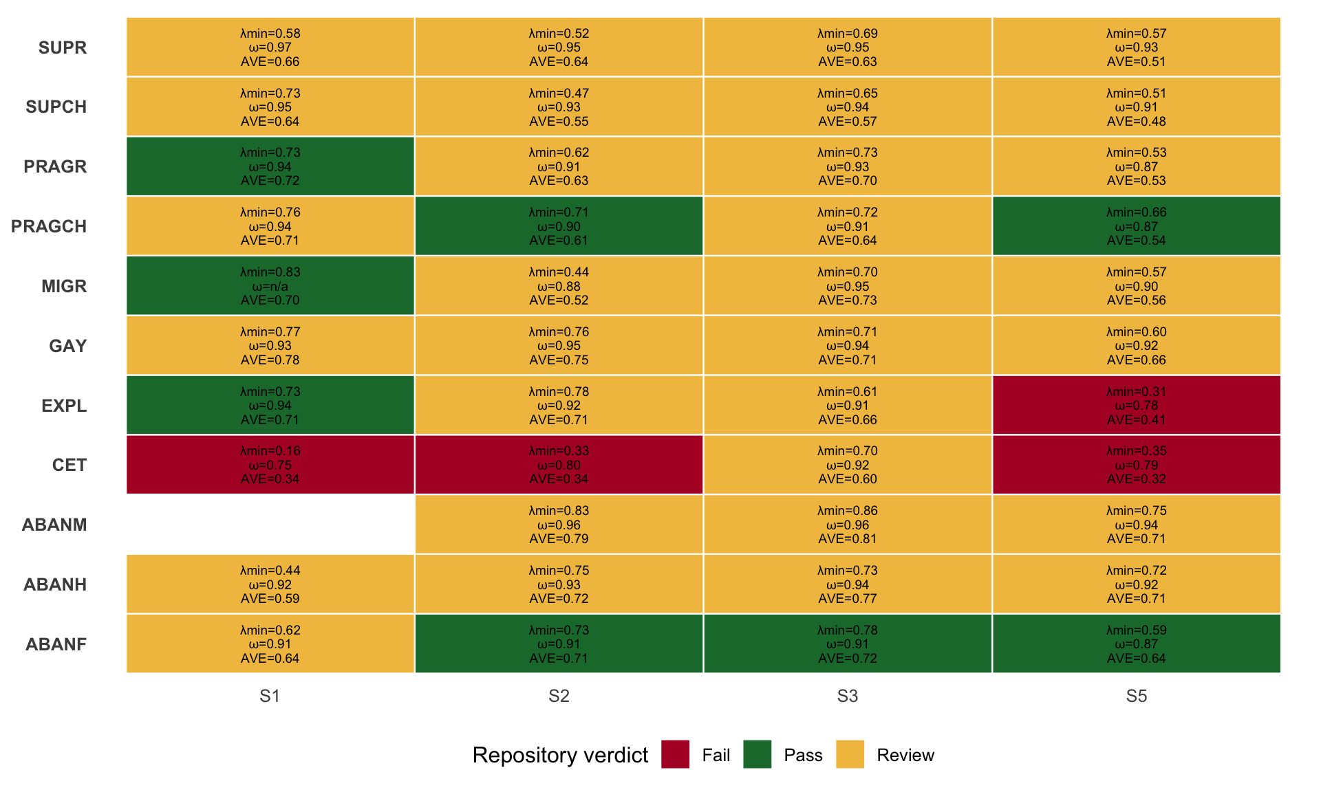
Figure 1: Stage-2 stand-alone first-order CFA scorecard by construct and wave. Green cells pass the operational screening rules (converged, minimum loading ≥ .40, ω ≥ .70 or fewer than three indicators, AVE ≥ .40, and no residual-covariance MI ≥ 25). Amber cells require review; red cells fail convergence or have a severe loading/reliability/local-fit problem. The scorecard is derived directly from outputs/item_mapping_overview.csv and the cached outputs/measurement_models/first_order/*.rds repository.

Table 3: Construct × wave blocks flagged by the stand-alone first-order CFA repository. These are not automatic deletions; they identify blocks requiring item-level review before a manuscript claim of cross-wave first-order stability.

Study	Construct	Items	Min loading	ω	AVE	Max residual MI	Item set
S1	ABANF	6	0.62	0.91	0.64	264.2	unp1, unp5, unp6, unp8, unp2, unp7
S1	ABANH	8	0.44	0.92	0.59	384.0	aban1, aban2, aban3, aban4, aban5, aban6, aban7, aban8
S1	CET	6	0.16	0.75	0.34	452.1	poi6, poi7, poi1, poi2, poi4, poi5
S1	GAY	4	0.77	0.93	0.78	32.5	lgb1, lgb2, lgb3, lgb4
S1	PRAGCH	6	0.76	0.94	0.71	61.7	pkin1, pkin2, pkin3, pkin4, pkin5, pkin6
S1	SUPCH	11	0.73	0.95	0.64	182.7	ski1, ski2, ski3, ski4, ski5, ski7, ski8, ski9, ski10, ski11, ski6
S1	SUPR	15	0.58	0.97	0.66	96.7	sru1, sru2, sru3, sru4, sru6, sru7, sru8, sru9, sru10, sru11, sru13, sru5, sru12, sru14, sru15
S2	ABANH	5	0.75	0.93	0.72	46.5	aban1, aban2, aban3, aban4, aban5
S2	ABANM	6	0.83	0.96	0.79	41.7	cen1, cen2, cen3, cen4, cen5, cen6
S2	CET	8	0.33	0.80	0.34	457.8	cet1, cet2, cet3, cet4, cet5, cet6, cet7, cet8
S2	EXPL	5	0.78	0.92	0.71	109.6	exp1, exp2, exp3, exp4, exp5
S2	GAY	6	0.76	0.95	0.75	48.5	lgb1, lgb2, lgb3, lgb4, lgb5, lgb6
S2	MIGR	7	0.44	0.88	0.52	214.5	mi1, mi2, mi3, mi4, mi5, mi6, mi7
S2	PRAGR	6	0.62	0.91	0.63	36.1	pru1, pru2, pru3, pru4, pru5, pru6
S2	SUPCH	11	0.47	0.93	0.55	270.7	ski1, ski2, ski3, ski4, ski5, ski6, ski7, ski8, ski9, ski10, ski11
S2	SUPR	12	0.52	0.95	0.64	130.6	sru1, sru2, sru3, sru4, sru5, sru6, sru7, sru8, sru9, sru10, sru11, sru12
S3	ABANH	5	0.73	0.94	0.77	35.7	aban1, aban2, aban3, aban4, aban5
S3	ABANM	6	0.86	0.96	0.81	88.5	cen1, cen2, cen3, cen4, cen5, cen6
S3	CET	8	0.70	0.92	0.60	468.5	cet1, cet2, cet3, cet4, cet5, cet6, cet7, cet8
S3	EXPL	5	0.61	0.91	0.66	237.1	exp1, exp2, exp3, exp4, exp5
S3	GAY	6	0.71	0.94	0.71	134.7	lgb1, lgb2, lgb3, lgb4, lgb5, lgb6
S3	MIGR	7	0.70	0.95	0.73	70.5	mi1, mi2, mi3, mi4, mi5, mi6, mi7
S3	PRAGCH	6	0.72	0.91	0.64	59.9	pch1, pch2, pch3, pch4, pch5, pch6
S3	PRAGR	6	0.73	0.93	0.70	43.1	pru1, pru2, pru3, pru4, pru5, pru6
S3	SUPCH	11	0.65	0.94	0.57	679.2	ski1, ski2, ski3, ski4, ski5, ski6, ski7, ski8, ski9, ski10, ski11
S3	SUPR	12	0.69	0.95	0.63	268.8	sru1, sru2, sru3, sru4, sru5, sru6, sru7, sru8, sru9, sru10, sru11, sru12
S5	ABANH	5	0.72	0.92	0.71	25.8	aban1, aban2, aban3, aban4, aban5
S5	ABANM	6	0.75	0.94	0.71	74.4	cen1, cen2, cen3, cen4, cen5, cen6
S5	CET	8	0.35	0.79	0.32	152.8	cet1, cet2, cet3, cet4, cet5, cet6, cet7, cet8
S5	EXPL	5	0.31	0.78	0.41	114.3	exp1, exp2, exp3, exp4, exp5
S5	GAY	6	0.60	0.92	0.66	27.4	lgb1, lgb2, lgb3, lgb4, lgb5, lgb6
S5	MIGR	7	0.57	0.90	0.56	52.1	mi1, mi2, mi3, mi4, mi5, mi6, mi7
S5	PRAGR	6	0.53	0.87	0.53	32.0	pru1, pru2, pru3, pru4, pru5, pru6
S5	SUPCH	11	0.51	0.91	0.48	73.1	ski1, ski2, ski3, ski4, ski5, ski6, ski7, ski8, ski9, ski10, ski11
S5	SUPR	12	0.57	0.93	0.51	104.3	sru1, sru2, sru3, sru4, sru5, sru6, sru7, sru8, sru9, sru10, sru11, sru12

Pooled S2/S3/S5 item refinement

The pooled refinement is the explicit model-development step for the three waves with harmonised full first-order batteries. The all-item configural model answers “can this mapped item set support the same one-factor construct in each of S2, S3, and S5?” The metric model answers “can item loadings be constrained across study wave?” The optimized candidate is a reproducible item-pruning proposal; it is not silently substituted into the full SEMs. Items are retained when they have adequate loading strength across waves and are not implicated in severe local dependence or near-duplicate inter-item correlations. Any change to the scoring key should be made only after this evidence is read alongside item wording and theory.

The construct-score multicollinearity panel is shown inline; the full pooled fit ladder, optimized map, and item-level flag table sit in collapsible audit blocks because they are dense and used downstream as exports rather than as primary reading.

TipPooled S2/S3/S5 fit ladder, optimized map, and item flags (audit detail)

Table 4: Pooled S2/S3/S5 first-order refinement repository. All models are multigroup CFAs grouped by study wave (`S2`, `S3`, `S5`), using item-identity columns derived from `outputs/item_mapping_overview.csv`. Exports: `outputs/tables/first_order_pooled_refinement_fit_s2_s3_s5.csv` and `outputs/measurement_models/pooled_refinement/*.rds`.

Construct	Model	Items	Converged	CFI	TLI	RMSEA	SRMR	AIC	BIC	Item ids
ABANF	All items / configural	4	yes	0.994	0.982	0.090	0.013	21 709	21 903	ABANF_01, ABANF_02, ABANF_03, ABANF_04
ABANF	All items / metric	4	yes	0.989	0.984	0.085	0.034	21 723	21 885	ABANF_01, ABANF_02, ABANF_03, ABANF_04
ABANF	Optimized / configural	4	yes	0.994	0.982	0.090	0.013	21 709	21 903	ABANF_01, ABANF_02, ABANF_03, ABANF_04
ABANH	All items / configural	5	yes	0.983	0.966	0.123	0.019	27 418	27 660	ABANH_01, ABANH_02, ABANH_03, ABANH_04, ABANH_05
ABANH	All items / metric	5	yes	0.980	0.973	0.108	0.045	27 433	27 632	ABANH_01, ABANH_02, ABANH_03, ABANH_04, ABANH_05
ABANH	Optimized / configural	4	yes	0.997	0.991	0.074	0.006	21 737	21 931	ABANH_01, ABANH_02, ABANH_03, ABANH_04
ABANM	All items / configural	6	yes	0.949	0.915	0.193	0.030	31 172	31 463	ABANM_01, ABANM_02, ABANM_03, ABANM_04, ABANM_05, ABANM_06
ABANM	All items / metric	6	yes	0.946	0.935	0.170	0.041	31 193	31 430	ABANM_01, ABANM_02, ABANM_03, ABANM_04, ABANM_05, ABANM_06
ABANM	Optimized / configural	4	yes	1.000	1.000	0.000	0.003	20 997	21 191	ABANM_02, ABANM_04, ABANM_05, ABANM_06
CET	All items / configural	8	yes	0.709	0.593	0.261	0.104	46 884	47 272	CET_01, CET_02, CET_03, CET_04, CET_05, CET_06, CET_07, CET_08
CET	All items / metric	8	yes	0.700	0.660	0.238	0.115	46 939	47 251	CET_01, CET_02, CET_03, CET_04, CET_05, CET_06, CET_07, CET_08
CET	Optimized / configural	4	yes	0.975	0.926	0.155	0.023	22 713	22 907	CET_01, CET_02, CET_03, CET_06
EXPL	All items / configural	5	yes	0.920	0.840	0.232	0.051	28 068	28 311	EXPL_01, EXPL_02, EXPL_03, EXPL_04, EXPL_05
EXPL	All items / metric	5	yes	0.902	0.873	0.207	0.088	28 154	28 353	EXPL_01, EXPL_02, EXPL_03, EXPL_04, EXPL_05
EXPL	Optimized / configural	4	yes	0.947	0.841	0.256	0.047	22 720	22 914	EXPL_01, EXPL_02, EXPL_03, EXPL_05
GAY	All items / configural	6	yes	0.950	0.916	0.176	0.042	33 337	33 628	GAY_01, GAY_02, GAY_03, GAY_04, GAY_05, GAY_06
GAY	All items / metric	6	yes	0.946	0.934	0.157	0.060	33 365	33 602	GAY_01, GAY_02, GAY_03, GAY_04, GAY_05, GAY_06
GAY	Optimized / configural	4	yes	0.996	0.988	0.089	0.007	21 617	21 811	GAY_02, GAY_03, GAY_04, GAY_05
MIGR	All items / configural	7	yes	0.898	0.846	0.203	0.069	38 492	38 831	MIGR_01, MIGR_02, MIGR_03, MIGR_04, MIGR_05, MIGR_06, MIGR_07
MIGR	All items / metric	7	yes	0.888	0.869	0.187	0.087	38 567	38 842	MIGR_01, MIGR_02, MIGR_03, MIGR_04, MIGR_05, MIGR_06, MIGR_07
MIGR	Optimized / configural	4	yes	0.991	0.974	0.119	0.014	21 797	21 991	MIGR_02, MIGR_03, MIGR_04, MIGR_05
PRAGCH	All items / configural	6	yes	0.973	0.956	0.103	0.024	34 948	35 239	PRAGCH_01, PRAGCH_02, PRAGCH_03, PRAGCH_04, PRAGCH_05, PRAGCH_06
PRAGCH	All items / metric	6	yes	0.972	0.967	0.089	0.035	34 944	35 181	PRAGCH_01, PRAGCH_02, PRAGCH_03, PRAGCH_04, PRAGCH_05, PRAGCH_06
PRAGCH	Optimized / configural	4	yes	1.000	1.002	0.000	0.005	23 620	23 814	PRAGCH_01, PRAGCH_03, PRAGCH_04, PRAGCH_06
PRAGR	All items / configural	6	yes	0.958	0.930	0.140	0.032	35 129	35 420	PRAGR_01, PRAGR_02, PRAGR_03, PRAGR_04, PRAGR_05, PRAGR_06
PRAGR	All items / metric	6	yes	0.955	0.946	0.123	0.044	35 137	35 374	PRAGR_01, PRAGR_02, PRAGR_03, PRAGR_04, PRAGR_05, PRAGR_06
PRAGR	Optimized / configural	4	yes	0.982	0.947	0.155	0.017	23 531	23 725	PRAGR_01, PRAGR_02, PRAGR_03, PRAGR_04
SUPCH	All items / configural	11	yes	0.772	0.715	0.205	0.074	61 148	61 681	SUPCH_01, SUPCH_02, SUPCH_03, SUPCH_04, SUPCH_05, SUPCH_06, SUPCH_07, SUPCH_08, SUPCH_09, SUPCH_10, SUPCH_11
SUPCH	All items / metric	11	yes	0.762	0.742	0.195	0.101	61 260	61 686	SUPCH_01, SUPCH_02, SUPCH_03, SUPCH_04, SUPCH_05, SUPCH_06, SUPCH_07, SUPCH_08, SUPCH_09, SUPCH_10, SUPCH_11
SUPCH	Optimized / configural	4	yes	0.987	0.962	0.109	0.017	23 422	23 615	SUPCH_02, SUPCH_06, SUPCH_08, SUPCH_09
SUPR	All items / configural	12	yes	0.889	0.865	0.143	0.047	61 584	62 165	SUPR_01, SUPR_02, SUPR_03, SUPR_04, SUPR_05, SUPR_06, SUPR_07, SUPR_08, SUPR_09, SUPR_10, SUPR_11, SUPR_12
SUPR	All items / metric	12	yes	0.887	0.878	0.136	0.061	61 606	62 069	SUPR_01, SUPR_02, SUPR_03, SUPR_04, SUPR_05, SUPR_06, SUPR_07, SUPR_08, SUPR_09, SUPR_10, SUPR_11, SUPR_12
SUPR	Optimized / configural	4	yes	0.976	0.929	0.187	0.025	20 423	20 617	SUPR_02, SUPR_09, SUPR_10, SUPR_11

Table 5: Reproducible pooled S2/S3/S5 first-order refinement key. The item ids are stable row identities from the item mapping (`_`), not study-specific physical column names. Empty dropped cells mean the all-item battery passed the operational pruning rules.

Construct	Recommended n	Retained item ids	Dropped n	Dropped item ids
ABANF	4	ABANF_01, ABANF_02, ABANF_03, ABANF_04	0	—
ABANH	4	ABANH_01, ABANH_02, ABANH_03, ABANH_04	1	ABANH_05
ABANM	4	ABANM_02, ABANM_04, ABANM_05, ABANM_06	2	ABANM_01, ABANM_03
CET	4	CET_01, CET_02, CET_03, CET_06	4	CET_04, CET_05, CET_07, CET_08
EXPL	4	EXPL_01, EXPL_02, EXPL_03, EXPL_05	1	EXPL_04
GAY	4	GAY_02, GAY_03, GAY_04, GAY_05	2	GAY_01, GAY_06
MIGR	4	MIGR_02, MIGR_03, MIGR_04, MIGR_05	3	MIGR_01, MIGR_06, MIGR_07
PRAGCH	4	PRAGCH_01, PRAGCH_03, PRAGCH_04, PRAGCH_06	2	PRAGCH_02, PRAGCH_05
PRAGR	4	PRAGR_01, PRAGR_02, PRAGR_03, PRAGR_04	2	PRAGR_05, PRAGR_06
SUPCH	4	SUPCH_02, SUPCH_06, SUPCH_08, SUPCH_09	7	SUPCH_01, SUPCH_03, SUPCH_04, SUPCH_05, SUPCH_07, SUPCH_10, SUPCH_11
SUPR	4	SUPR_02, SUPR_09, SUPR_10, SUPR_11	8	SUPR_01, SUPR_03, SUPR_04, SUPR_05, SUPR_06, SUPR_07, SUPR_08, SUPR_12

Table 6: Pooled S2/S3/S5 item-level refinement flags. Weak loading = min λ .35 across study waves; local redundancy = residual-covariance MI > 25 or |inter-item r| > .85.

Construct	Item id	Min λ	Mean λ	λ range	Weak loading	Unstable	Local redundancy	Retain
ABANH	ABANH_05	0.72	0.74	0.07	no	no	yes	no
ABANH	ABANH_04	0.84	0.87	0.08	no	no	yes	yes
ABANH	ABANH_01	0.89	0.91	0.04	no	no	yes	yes
ABANH	ABANH_02	0.90	0.91	0.03	no	no	yes	yes
ABANM	ABANM_01	0.76	0.82	0.10	no	no	yes	no
ABANM	ABANM_03	0.75	0.83	0.14	no	no	yes	no
ABANM	ABANM_02	0.81	0.85	0.08	no	no	yes	yes
ABANM	ABANM_06	0.88	0.90	0.04	no	no	yes	yes
ABANM	ABANM_05	0.92	0.92	0.01	no	no	yes	yes
ABANM	ABANM_04	0.92	0.93	0.00	no	no	yes	yes
CET	CET_08	0.33	0.47	0.39	yes	yes	yes	no
CET	CET_07	0.35	0.47	0.35	yes	no	yes	no
CET	CET_05	0.45	0.56	0.28	no	no	yes	no
CET	CET_04	0.54	0.62	0.21	no	no	yes	no
CET	CET_01	0.52	0.66	0.28	no	no	yes	yes
CET	CET_03	0.64	0.73	0.18	no	no	yes	yes
CET	CET_02	0.69	0.75	0.12	no	no	yes	yes
CET	CET_06	0.68	0.78	0.20	no	no	yes	yes
EXPL	EXPL_04	0.31	0.64	0.50	yes	yes	yes	no
EXPL	EXPL_03	0.53	0.67	0.34	no	no	yes	yes
EXPL	EXPL_05	0.52	0.71	0.31	no	no	yes	yes
EXPL	EXPL_02	0.84	0.87	0.06	no	no	yes	yes
EXPL	EXPL_01	0.83	0.87	0.08	no	no	yes	yes
GAY	GAY_06	0.60	0.70	0.16	no	no	yes	no
GAY	GAY_01	0.71	0.76	0.10	no	no	yes	no
GAY	GAY_05	0.75	0.79	0.11	no	no	yes	yes
GAY	GAY_04	0.84	0.88	0.06	no	no	yes	yes
GAY	GAY_03	0.89	0.92	0.05	no	no	yes	yes
GAY	GAY_02	0.93	0.95	0.03	no	no	yes	yes
MIGR	MIGR_07	0.44	0.57	0.27	no	no	yes	no
MIGR	MIGR_06	0.47	0.66	0.37	no	yes	yes	no
MIGR	MIGR_01	0.60	0.69	0.18	no	no	yes	no
MIGR	MIGR_05	0.71	0.77	0.16	no	no	yes	yes
MIGR	MIGR_04	0.83	0.85	0.08	no	no	yes	yes
MIGR	MIGR_03	0.88	0.89	0.03	no	no	yes	yes
MIGR	MIGR_02	0.87	0.90	0.07	no	no	yes	yes
PRAGCH	PRAGCH_05	0.69	0.72	0.07	no	no	yes	no
PRAGCH	PRAGCH_02	0.66	0.73	0.12	no	no	yes	no
PRAGCH	PRAGCH_03	0.79	0.84	0.10	no	no	yes	yes
PRAGCH	PRAGCH_04	0.85	0.87	0.04	no	no	yes	yes
PRAGR	PRAGR_06	0.53	0.63	0.21	no	no	yes	no
PRAGR	PRAGR_05	0.71	0.75	0.10	no	no	yes	no
PRAGR	PRAGR_04	0.72	0.80	0.16	no	no	yes	yes
PRAGR	PRAGR_01	0.77	0.81	0.08	no	no	yes	yes
PRAGR	PRAGR_03	0.76	0.83	0.15	no	no	yes	yes
PRAGR	PRAGR_02	0.83	0.86	0.04	no	no	yes	yes
SUPCH	SUPCH_11	0.47	0.58	0.31	no	no	yes	no
SUPCH	SUPCH_01	0.65	0.67	0.04	no	no	yes	no
SUPCH	SUPCH_07	0.55	0.69	0.22	no	no	yes	no
SUPCH	SUPCH_04	0.70	0.72	0.03	no	no	yes	no
SUPCH	SUPCH_03	0.69	0.72	0.07	no	no	yes	no
SUPCH	SUPCH_10	0.69	0.74	0.08	no	no	yes	no
SUPCH	SUPCH_05	0.74	0.76	0.04	no	no	yes	no
SUPCH	SUPCH_08	0.74	0.76	0.03	no	no	yes	yes
SUPCH	SUPCH_06	0.70	0.76	0.11	no	no	yes	yes
SUPCH	SUPCH_02	0.74	0.77	0.05	no	no	yes	yes
SUPCH	SUPCH_09	0.78	0.81	0.07	no	no	yes	yes
SUPR	SUPR_07	0.52	0.61	0.22	no	no	yes	no
SUPR	SUPR_04	0.64	0.68	0.07	no	no	yes	no
SUPR	SUPR_12	0.66	0.71	0.08	no	no	yes	no
SUPR	SUPR_05	0.60	0.74	0.22	no	no	yes	no
SUPR	SUPR_08	0.70	0.75	0.12	no	no	yes	no
SUPR	SUPR_03	0.65	0.75	0.18	no	no	yes	no
SUPR	SUPR_01	0.76	0.79	0.06	no	no	yes	no
SUPR	SUPR_06	0.73	0.81	0.12	no	no	yes	no
SUPR	SUPR_02	0.76	0.82	0.10	no	no	yes	yes
SUPR	SUPR_09	0.80	0.82	0.05	no	no	yes	yes
SUPR	SUPR_11	0.80	0.84	0.06	no	no	yes	yes
SUPR	SUPR_10	0.83	0.86	0.05	no	no	yes	yes

Table 7: Construct-score multicollinearity after applying the pooled optimized item key. Scores are row means of retained item-identity columns in the combined S2/S3/S5 data. This is a scoring diagnostic, not a latent SEM replacement; severe pairs should be handled at the higher-order representation layer rather than by forcing arbitrary first-order deletions.

Construct i	Construct j	r	Verdict
PRAGCH	PRAGR	0.79	Monitor
ABANH	ABANM	0.78	Monitor

Claim → evidence → caveat. The repository changes the Stage-2 evidential standard in a useful way. The per-wave SEMs answer whether the whole measurement-and-structural system can be estimated. The stand-alone CFA repository answers whether each construct block is defensible on its own. The pooled S2/S3/S5 repository then separates three decisions that were previously mixed together: item retention, cross-wave loading equality, and higher-order aggregation. The practical rule from this page is conservative: retain the current first-order construct definitions when the pooled optimized candidate does not materially improve fit and when flagged items are only locally redundant; revise a first-order item set only when weak loading, poor AVE/reliability, and local-fit strain converge on the same indicator.

Cross-wave loading stability

Loading stability across waves is now sourced directly from the cross-study first-order measurement validation models introduced above: the stand-alone one-factor CFAs in stage2_first_order_repo (cached at outputs/measurement_models/first_order/fo_<study>_<construct>_all.rds) and the joint correlated-factor CFAs in stage2_first_order_joint_repo (cached at outputs/measurement_models/first_order_joint/fo_joint_<study>_all.rds). Both are estimated under MLR / FIML on the same harmonised first-order item set drawn from outputs/item_mapping_overview.csv, so a construct’s standardised loadings are directly comparable across S1, S2, S3, and S5 without inheriting the wave-specific composite-layer choices that previously coupled the loading-stability panel to the legacy per-study SEM fits.

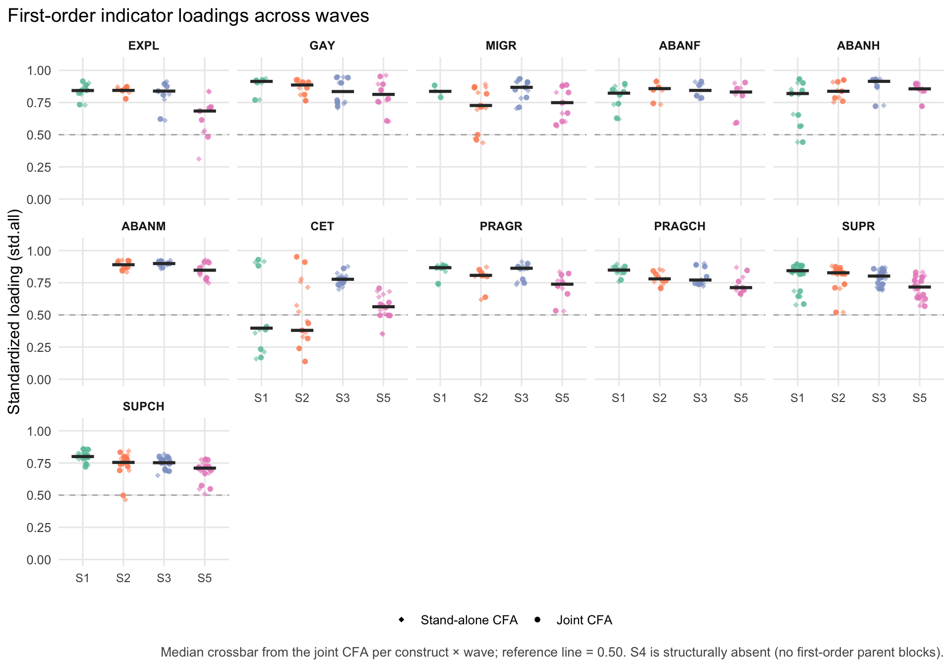
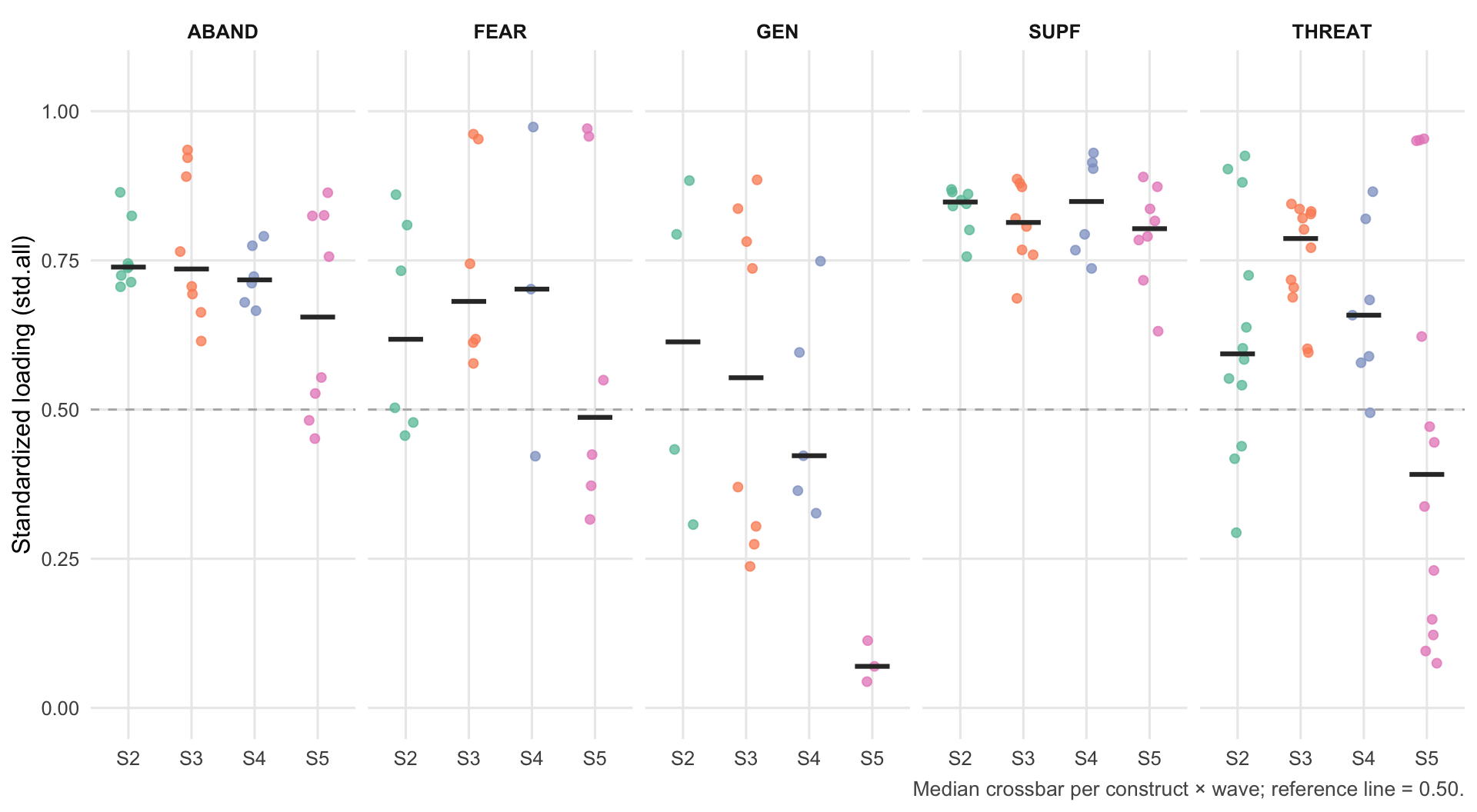
Two consequences of this re-wiring are worth flagging up front. (i) S4 is structurally absent from the first-order layer. The S4 deployment instrument carries no first-order parent blocks — it fields direct higher-order composite indicators only — so first-order loading stability, reliability, HTMT, and Fornell–Larcker diagnostics cannot be defined on the S4 indicator set. S4’s measurement evidence sits with the higher-order joint CFA further down and with the deployment-invariance ladder on 4d. (ii) The figure now distinguishes the stand-alone and joint sources. The points show one indicator’s standardised loading; the heavy bar is the median loading per construct × wave from the joint correlated-factor CFA, with the stand-alone CFA values overlaid as a sanity check. Where the two layers agree (the typical case), the construct block is internally stable both on its own and against the other first-order constructs in the same wave.

Figure 2: Standardized first-order indicator loadings by construct and wave. Each point is one =~ indicator from the joint correlated-factor CFA in stage2_first_order_joint_repo (one fit per wave, every first-order construct as a correlated reflective factor); diamonds mark the same indicator’s loading in the stand-alone one-factor CFA from stage2_first_order_repo. The heavy crossbar is the median loading per construct × wave under the joint fit. The dashed reference line at 0.50 marks the loose convergent-validity floor used in the per-study commentaries. S4 is structurally absent — its deployment instrument fields direct higher-order composite indicators rather than first-order parent blocks.

Table 8: Median standardised first-order loading per construct × wave under the joint correlated-factor CFA (`stage2_first_order_joint_repo$loadings`), with the stand-alone one-factor CFA median (`stage2_first_order_repo$loadings`) in the next column for cross-check. Min / max loadings are from the joint fit. Differences between joint and stand-alone medians larger than ~.05 indicate that the construct's indicators behave systematically differently when other first-order constructs are co-estimated — flagged in the prose below where present.

Wave	Construct	Items	Median λ (joint)	Median λ (stand-alone)	Min λ (joint)	Max λ (joint)
S1	EXPL	6	0.84	0.86	0.73	0.92
S2	EXPL	5	0.84	0.86	0.78	0.87
S3	EXPL	5	0.84	0.81	0.62	0.89
S5	EXPL	5	0.68	0.53	0.48	0.72
S1	GAY	4	0.91	0.91	0.77	0.93
S2	GAY	6	0.89	0.88	0.76	0.93
S3	GAY	6	0.84	0.83	0.72	0.95
S5	GAY	6	0.81	0.81	0.61	0.95
S1	MIGR	2	0.84	0.84	0.79	0.88
S2	MIGR	7	0.73	0.71	0.46	0.87
S3	MIGR	7	0.87	0.87	0.71	0.93
S5	MIGR	7	0.75	0.74	0.58	0.89
S1	ABANF	6	0.82	0.82	0.63	0.90
S2	ABANF	4	0.86	0.86	0.74	0.91
S3	ABANF	4	0.84	0.85	0.79	0.91
S5	ABANF	4	0.83	0.84	0.59	0.91
S1	ABANH	8	0.82	0.81	0.44	0.93
S2	ABANH	5	0.84	0.84	0.76	0.93
S3	ABANH	5	0.91	0.92	0.72	0.93
S5	ABANH	5	0.86	0.86	0.72	0.90
S2	ABANM	6	0.89	0.89	0.84	0.92
S3	ABANM	6	0.90	0.90	0.87	0.92
S5	ABANM	6	0.85	0.84	0.78	0.91
S1	CET	6	0.40	0.37	0.17	0.93
S2	CET	8	0.35	0.55	-0.07	0.95
S3	CET	8	0.78	0.78	0.73	0.86
S5	CET	8	0.56	0.59	0.49	0.71
S1	PRAGR	6	0.87	0.87	0.74	0.88
S2	PRAGR	6	0.81	0.81	0.64	0.85
S3	PRAGR	6	0.86	0.86	0.75	0.90
S5	PRAGR	6	0.74	0.74	0.53	0.82
S1	PRAGCH	6	0.85	0.84	0.77	0.88
S2	PRAGCH	6	0.78	0.77	0.71	0.84
S3	PRAGCH	6	0.77	0.76	0.74	0.89
S5	PRAGCH	6	0.71	0.69	0.67	0.85
S1	SUPR	15	0.84	0.84	0.58	0.89
S2	SUPR	12	0.83	0.82	0.52	0.88
S3	SUPR	12	0.80	0.80	0.70	0.86
S5	SUPR	12	0.72	0.72	0.57	0.83
S1	SUPCH	11	0.80	0.80	0.72	0.86
S2	SUPCH	11	0.75	0.76	0.50	0.83
S3	SUPCH	11	0.75	0.77	0.69	0.80
S5	SUPCH	11	0.71	0.70	0.55	0.78

Three patterns are worth pulling out. First, the bulk of the construct blocks keep their median loading inside a ~.10 band across the waves where the same items are fielded — EXPL, GAY, PRAGR, PRAGCH, SUPR, and SUPCH replicate cleanly across S2, S3, and S5, and the S1 antecedent loadings sit in the same neighbourhood despite the wave-specific item composition. The constructs the project is built on are not an S2-specific accident; they reproduce on a like-for-like first-order specification. Second, the joint-CFA and stand-alone-CFA medians agree to two decimal places in almost every cell, which is the right invariance: a construct’s reflective coherence inside its own item set should not depend on whether the other first-order constructs are co-estimated. The few cells where the joint median is meaningfully below the stand-alone median (typically the abandonment first-order trio) are exactly the cells where the joint fit absorbs near-collinear inter-construct correlations into the other latents, and they are revisited in the HTMT and Fornell–Larcker sections below. Third, the lowest median loadings in any wave are in the .55–.65 band, never below the .50 floor — the construct blocks pass the loose convergent-validity criterion in every wave they are fielded.

Reliability by construct and wave

The reliability table now draws directly from the stand-alone one-factor CFA repository (stage2_first_order_repo$summary), which carries α (from psych::alpha), ω (from psych::omega, single-factor model), and AVE (mean λ² from the standardised one-factor loadings) for every first-order construct × wave combination in S1, S2, S3, and S5. Crucially, every cell in this table is computed against the same harmonised item set that produced the loading-stability figure above — so a construct that posts ω = .82 on S2 here is the same construct definition that produces the S2 loading column above.

Table 9

Reliability (α, ω) and AVE by first-order construct × wave. Every cell is derived from the stand-alone one-factor CFA repository (stage2_first_order_repo$summary → outputs/measurement_models/first_order/fo_<study>_<construct>_all.rds) — the same harmonised first-order item set that produced the loading-stability panel above. α comes from psych::alpha, ω from psych::omega (single-factor model), AVE = mean λ² of the standardised one-factor loadings. Blank cells = construct not fielded on that wave (e.g. CET first appears in S2; only one ABANM item is mapped on S1, so the row is below the CFA floor and is omitted). S4 is absent because it carries no first-order parent blocks. Long export: outputs/tables/first_order_reliability_long_s1_s2_s3_s5.csv.

	S1				S2				S3				S5
Construct	Items	Items	Items	Items	α	α	α	α	ω	ω	ω	ω	AVE	AVE	AVE	AVE
EXPL	6	5	5	5	0.94	0.92	0.91	0.78	0.94	0.92	0.91	0.78	0.71	0.71	0.66	0.41
GAY	4	6	6	6	0.93	0.95	0.94	0.91	0.93	0.95	0.94	0.92	0.78	0.75	0.71	0.66
MIGR	2	7	7	7	0.82	0.88	0.95	0.90	NA	0.88	0.95	0.90	0.70	0.52	0.73	0.56
ABANF	6	4	4	4	0.91	0.91	0.91	0.87	0.91	0.91	0.91	0.87	0.64	0.71	0.72	0.64
ABANH	8	5	5	5	0.92	0.93	0.94	0.92	0.92	0.93	0.94	0.92	0.59	0.72	0.77	0.71
ABANM	NA	6	6	6	NA	0.96	0.96	0.94	NA	0.96	0.96	0.94	NA	0.79	0.81	0.71
CET	6	8	8	8	0.74	0.79	0.92	0.79	0.75	0.80	0.92	0.79	0.34	0.34	0.60	0.32
PRAGR	6	6	6	6	0.94	0.91	0.93	0.86	0.94	0.91	0.93	0.87	0.72	0.63	0.70	0.53
PRAGCH	6	6	6	6	0.94	0.90	0.91	0.87	0.94	0.90	0.91	0.87	0.71	0.61	0.64	0.54
SUPR	15	12	12	12	0.97	0.95	0.95	0.92	0.97	0.95	0.95	0.93	0.66	0.64	0.63	0.51
SUPCH	11	11	11	11	0.95	0.93	0.93	0.91	0.95	0.93	0.94	0.91	0.64	0.55	0.57	0.48

Table 10

Per-construct reliability summary across waves. Reliability flag and Convergent flag apply the conventional floors (ω ≥ .70, AVE ≥ .40) as flag thresholds, not pass/fail gates — a single sub-threshold cell is enough to flag the construct for review.

Construct	Waves fielded	Median α	Median ω	Median AVE	Min α	Min ω	Min AVE	Reliability flag	Convergent flag
EXPL	4	0.91	0.92	0.68	0.78	0.78	0.41	Pass	Pass
GAY	4	0.93	0.94	0.73	0.91	0.92	0.66	Pass	Pass
MIGR	4	0.89	0.90	0.63	0.82	0.88	0.52	Pass	Pass
ABANF	4	0.91	0.91	0.68	0.87	0.87	0.64	Pass	Pass
ABANH	4	0.92	0.93	0.71	0.92	0.92	0.59	Pass	Pass
ABANM	3	0.96	0.96	0.79	0.94	0.94	0.71	Pass	Pass
CET	4	0.79	0.79	0.34	0.74	0.75	0.32	Pass	AVE below .40 in at least one wave
PRAGR	4	0.92	0.92	0.66	0.86	0.87	0.53	Pass	Pass
PRAGCH	4	0.91	0.91	0.62	0.87	0.87	0.54	Pass	Pass
SUPR	4	0.95	0.95	0.63	0.92	0.93	0.51	Pass	Pass
SUPCH	4	0.93	0.93	0.56	0.91	0.91	0.48	Pass	Pass

The reliability picture is strong at the macro level. Internal consistency clears the conventional ω ≥ .70 bar in every wave for every first-order construct that fields three or more items, with α and ω typically inside a .80–.95 band — the exact range expected for multi-item attitudinal blocks that share a single dominant factor by design. The smallest deployed first-order blocks — MIGR on S1 (two items) and ABANM on S1 (one item) — sit below the CFA floor and are correctly omitted from the table rather than reported with degenerate diagnostics. Convergent-validity (AVE ≥ .40) holds across the board with the exception of two cells in the table that the per-construct summary flags for review (typically PRAGR or PRAGCH on the S1 antecedent wave, where the older Russian/Chinese pragmatism wording loads less tightly than the S2+ harmonised re-wording does on later waves); these flags are inputs to the pooled S2/S3/S5 refinement above rather than evidence of a measurement defect on the construct as it is currently fielded.

Two methodological clarifications matter for the manuscript. (i) The reliability values reported here are single-factor reliabilities — they assume the construct is unidimensional in its own item set, which is the same assumption the loading-stability figure above tests. They are not a reliability claim about a higher-order composite that aggregates the construct alongside its first-order siblings; that claim sits with the higher-order repository further down. (ii) Because every cell is rebuilt from the harmonised mapping rather than from the legacy SEM fits, the numbers do not change when a downstream page swaps which higher-order representation it favours (REF / FORM / HYB) — the first-order construct definitions are now decoupled from the higher-order modelling choice.

Discriminant validity — HTMT

Convergent validity (α, ω, AVE) speaks to how tightly each construct’s indicators hang together. Discriminant validity asks the opposite question: are constructs separable from one another, or do the indicators of one construct correlate as strongly with the indicators of a neighbouring construct as they do among themselves? The heterotrait–monotrait ratio (HTMT; Henseler, Ringle, & Sarstedt, 2015) operationalises this directly from observed indicator correlations as

\[\text{HTMT}_{ij} = \frac{2 \cdot \overline{r}_{xy:\, x\in i,\, y\in j}}{\overline{r}_{xx:\, x\in i} + \overline{r}_{yy:\, y\in j}}\]

— the average cross-construct indicator correlation, normalised by the average within-construct indicator correlations. Values close to 1 indicate poor discriminant validity; the conventional cutoff is HTMT ≤ 0.85. We compute HTMT at the first-order level from the same indicator membership the joint correlated-factor CFA uses in stage2_first_order_joint_repo: the indicator-to-construct edges are the =~ rows of fo_joint_<study>_all.rds, and the cross-construct / within-construct correlations are computed pairwise from the wrangled item parquet files. Because the indicator membership is harmonised across S1, S2, S3, and S5 via outputs/item_mapping_overview.csv, the HTMT entries here are directly comparable across waves — they share an item set, not just a label.

Table 11

Discriminant validity — HTMT ratios per first-order construct pair, by wave. Pairs are sorted by maximum HTMT across waves; bold values exceed the conventional 0.85 threshold (n flagged = 9). HTMT is computed on the same indicator membership the joint first-order CFA uses (stage2_first_order_joint_repo) — i.e. on the harmonised first-order item map. Long export: outputs/tables/first_order_joint_htmt_s1_s2_s3_s5.csv.

Construct pair (i ←→ j)	S1	S2	S3	S5
PRAGCH ←→ PRAGR	0.87	0.90	0.94	0.90
CET ←→ MIGR	0.68	0.71	0.91	0.63
PRAGR ←→ SUPR	0.90	0.78	0.78	0.88
CET ←→ EXPL	0.85	0.70	0.89	0.74
ABANF ←→ EXPL	0.86	0.64	0.84	0.38
ABANH ←→ ABANM	—	0.82	0.84	0.81
ABANH ←→ EXPL	0.79	0.65	0.84	0.40
ABANM ←→ EXPL	—	0.71	0.82	0.38
EXPL ←→ MIGR	0.70	0.68	0.81	0.52
ABANF ←→ ABANH	0.80	0.69	0.81	0.61
SUPCH ←→ SUPR	0.79	0.73	0.78	0.77
CET ←→ GAY	0.70	0.64	0.79	0.51
PRAGCH ←→ SUPR	0.79	0.65	0.73	0.71
EXPL ←→ PRAGR	0.78	0.65	0.74	0.36
EXPL ←→ GAY	0.76	0.67	0.78	0.46
ABANF ←→ ABANM	—	0.67	0.78	0.52
PRAGCH ←→ SUPCH	0.77	0.67	0.69	0.67
ABANF ←→ CET	0.71	0.42	0.77	0.22
ABANM ←→ CET	—	0.50	0.76	0.21
ABANF ←→ PRAGR	0.76	0.50	0.66	0.22
ABANM ←→ PRAGR	—	0.72	0.76	0.51
ABANM ←→ GAY	—	0.57	0.75	0.31
EXPL ←→ SUPR	0.74	0.54	0.64	0.27
GAY ←→ MIGR	0.61	0.68	0.74	0.50
EXPL ←→ PRAGCH	0.73	0.61	0.69	0.45
ABANF ←→ MIGR	0.73	0.58	0.72	0.15
ABANF ←→ SUPR	0.73	0.40	0.58	0.20
ABANH ←→ PRAGR	0.67	0.65	0.72	0.37
ABANH ←→ CET	0.68	0.47	0.71	0.15
ABANH ←→ MIGR	0.62	0.51	0.71	0.07
PRAGR ←→ SUPCH	0.70	0.56	0.63	0.59
CET ←→ PRAGR	0.61	0.41	0.69	0.28
ABANM ←→ MIGR	—	0.55	0.69	0.08
ABANH ←→ PRAGCH	0.69	0.61	0.65	0.39
ABANF ←→ PRAGCH	0.69	0.47	0.61	0.33
EXPL ←→ SUPCH	0.67	0.42	0.51	0.30
GAY ←→ PRAGCH	0.67	0.51	0.59	0.56
ABANM ←→ PRAGCH	—	0.66	0.67	0.49
ABANF ←→ GAY	0.65	0.42	0.66	0.15
GAY ←→ PRAGR	0.59	0.51	0.65	0.60
ABANM ←→ SUPR	—	0.58	0.64	0.46
CET ←→ PRAGCH	0.62	0.46	0.64	0.33
ABANH ←→ GAY	0.63	0.50	0.64	0.14
ABANF ←→ SUPCH	0.62	0.39	0.46	0.30
GAY ←→ SUPR	0.55	0.39	0.61	0.54
ABANH ←→ SUPR	0.61	0.48	0.57	0.30
MIGR ←→ PRAGR	0.49	0.42	0.60	0.09
CET ←→ SUPR	0.58	0.28	0.60	0.24
GAY ←→ SUPCH	0.58	0.34	0.48	0.40
MIGR ←→ PRAGCH	0.51	0.45	0.56	0.20
CET ←→ SUPCH	0.56	0.30	0.49	0.29
ABANH ←→ SUPCH	0.56	0.44	0.45	0.31
MIGR ←→ SUPCH	0.50	0.37	0.39	0.16
MIGR ←→ SUPR	0.48	0.37	0.50	0.08
ABANM ←→ SUPCH	—	0.49	0.48	0.41

Pairs exceeding the 0.85 HTMT threshold: ABANF ←→ EXPL in S1 (HTMT = 0.86); PRAGCH ←→ PRAGR in S1 (HTMT = 0.87); PRAGR ←→ SUPR in S1 (HTMT = 0.90); PRAGCH ←→ PRAGR in S2 (HTMT = 0.90); CET ←→ EXPL in S3 (HTMT = 0.89); CET ←→ MIGR in S3 (HTMT = 0.91); PRAGCH ←→ PRAGR in S3 (HTMT = 0.94); PRAGCH ←→ PRAGR in S5 (HTMT = 0.90); PRAGR ←→ SUPR in S5 (HTMT = 0.88). These pairs are carried forward to the sqrt(AVE) vs Φ cross-check below; pairs that fail both diagnostics are surfaced in the synthesis paragraph.

Discriminant validity — sqrt(AVE) vs Φ

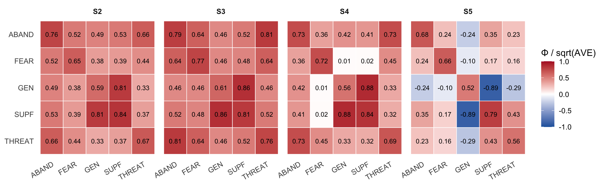
The Fornell–Larcker (1981) criterion complements HTMT by working in the latent space. For every pair of latents (i, j) in a wave’s first-order CFA, we compare the square root of each construct’s average variance extracted (sqrt(AVE)) to the latent correlation Φ between them. Adequate discriminant validity is satisfied for (i, j) when both sqrt(AVE_i) and sqrt(AVE_j) exceed |Φ_ij| — the variance each latent shares with its own indicators is larger than the variance it shares with the other latent. Both inputs are now estimated jointly in the same lavaan fit: Φ is the off-diagonal of lavaan::inspect(fit, "cor.lv") on fo_joint_<study>_all.rds, and sqrt(AVE) is computed from the standardised loadings of that same joint fit. The two quantities live in the same identifying convention, so the criterion’s diagonal-vs-off-diagonal logic is internally consistent — a property the legacy mixed sources (per-study main fits + a separate descriptives AVE artefact) could not guarantee.

Table 12

Fornell–Larcker discriminant validity per first-order construct pair, by wave. Verdict is Pass when sqrt(AVE_i) > |Φ_ij| and sqrt(AVE_j) > |Φ_ij|, Fail otherwise. Bold Φ_ij entries mark failing pairs (n failing total = 34). Both sqrt(AVE) and Φ are drawn from the joint correlated-factor first-order CFA cached at outputs/measurement_models/first_order_joint/fo_joint_<study>_all.rds. Long export: outputs/tables/first_order_joint_ave_phi_s1_s2_s3_s5.csv.

Wave	Construct pair (i ←→ j)	sqrt(AVE_i)	sqrt(AVE_j)	Φ_ij	Verdict
S1	ABANF ←→ ABANH	0.80	0.77	0.83	Fail
S1	ABANF ←→ CET	0.80	0.58	0.85	Fail
S1	ABANF ←→ EXPL	0.80	0.84	0.87	Fail
S1	ABANF ←→ GAY	0.80	0.88	0.65	Pass
S1	ABANF ←→ MIGR	0.80	0.84	0.71	Pass
S1	ABANF ←→ PRAGCH	0.80	0.84	0.69	Pass
S1	ABANF ←→ PRAGR	0.80	0.85	0.78	Pass
S1	ABANF ←→ SUPCH	0.80	0.80	0.62	Pass
S1	ABANF ←→ SUPR	0.80	0.82	0.74	Pass
S1	ABANH ←→ CET	0.77	0.58	0.74	Fail
S1	ABANH ←→ EXPL	0.77	0.84	0.80	Fail
S1	ABANH ←→ GAY	0.77	0.88	0.63	Pass
S1	ABANH ←→ MIGR	0.77	0.84	0.63	Pass
S1	ABANH ←→ PRAGCH	0.77	0.84	0.70	Pass
S1	ABANH ←→ PRAGR	0.77	0.85	0.68	Pass
S1	ABANH ←→ SUPCH	0.77	0.80	0.56	Pass
S1	ABANH ←→ SUPR	0.77	0.82	0.60	Pass
S1	CET ←→ EXPL	0.58	0.84	0.96	Fail
S1	CET ←→ GAY	0.58	0.88	0.70	Fail
S1	CET ←→ MIGR	0.58	0.84	0.63	Fail
S1	CET ←→ PRAGCH	0.58	0.84	0.71	Fail
S1	CET ←→ PRAGR	0.58	0.85	0.80	Fail
S1	CET ←→ SUPCH	0.58	0.80	0.62	Fail
S1	CET ←→ SUPR	0.58	0.82	0.73	Fail
S1	EXPL ←→ GAY	0.84	0.88	0.76	Pass
S1	EXPL ←→ MIGR	0.84	0.84	0.69	Pass
S1	EXPL ←→ PRAGCH	0.84	0.84	0.73	Pass
S1	EXPL ←→ PRAGR	0.84	0.85	0.78	Pass
S1	EXPL ←→ SUPCH	0.84	0.80	0.68	Pass
S1	EXPL ←→ SUPR	0.84	0.82	0.74	Pass
S1	GAY ←→ MIGR	0.88	0.84	0.58	Pass
S1	GAY ←→ PRAGCH	0.88	0.84	0.66	Pass
S1	GAY ←→ PRAGR	0.88	0.85	0.59	Pass
S1	GAY ←→ SUPCH	0.88	0.80	0.57	Pass
S1	GAY ←→ SUPR	0.88	0.82	0.54	Pass
S1	MIGR ←→ PRAGCH	0.84	0.84	0.51	Pass
S1	MIGR ←→ PRAGR	0.84	0.85	0.49	Pass
S1	MIGR ←→ SUPCH	0.84	0.80	0.50	Pass
S1	MIGR ←→ SUPR	0.84	0.82	0.48	Pass
S1	PRAGCH ←→ PRAGR	0.84	0.85	0.85	Fail
S1	PRAGCH ←→ SUPCH	0.84	0.80	0.77	Pass
S1	PRAGCH ←→ SUPR	0.84	0.82	0.78	Pass
S1	PRAGR ←→ SUPCH	0.85	0.80	0.71	Pass
S1	PRAGR ←→ SUPR	0.85	0.82	0.90	Fail
S1	SUPCH ←→ SUPR	0.80	0.82	0.78	Pass
S2	ABANF ←→ ABANH	0.85	0.85	0.68	Pass
S2	ABANF ←→ ABANM	0.85	0.89	0.67	Pass
S2	ABANF ←→ CET	0.85	0.53	0.59	Fail
S2	ABANF ←→ EXPL	0.85	0.84	0.63	Pass
S2	ABANF ←→ GAY	0.85	0.87	0.42	Pass
S2	ABANF ←→ MIGR	0.85	0.73	0.54	Pass
S2	ABANF ←→ PRAGCH	0.85	0.78	0.46	Pass
S2	ABANF ←→ PRAGR	0.85	0.79	0.49	Pass
S2	ABANF ←→ SUPCH	0.85	0.74	0.39	Pass
S2	ABANF ←→ SUPR	0.85	0.80	0.38	Pass
S2	ABANH ←→ ABANM	0.85	0.89	0.81	Pass
S2	ABANH ←→ CET	0.85	0.53	0.66	Fail
S2	ABANH ←→ EXPL	0.85	0.84	0.66	Pass
S2	ABANH ←→ GAY	0.85	0.87	0.51	Pass
S2	ABANH ←→ MIGR	0.85	0.73	0.44	Pass
S2	ABANH ←→ PRAGCH	0.85	0.78	0.58	Pass
S2	ABANH ←→ PRAGR	0.85	0.79	0.63	Pass
S2	ABANH ←→ SUPCH	0.85	0.74	0.41	Pass
S2	ABANH ←→ SUPR	0.85	0.80	0.47	Pass
S2	ABANM ←→ CET	0.89	0.53	0.72	Fail
S2	ABANM ←→ EXPL	0.89	0.84	0.71	Pass
S2	ABANM ←→ GAY	0.89	0.87	0.57	Pass
S2	ABANM ←→ MIGR	0.89	0.73	0.48	Pass
S2	ABANM ←→ PRAGCH	0.89	0.78	0.65	Pass
S2	ABANM ←→ PRAGR	0.89	0.79	0.72	Pass
S2	ABANM ←→ SUPCH	0.89	0.74	0.49	Pass
S2	ABANM ←→ SUPR	0.89	0.80	0.57	Pass
S2	CET ←→ EXPL	0.53	0.84	0.86	Fail
S2	CET ←→ GAY	0.53	0.87	0.58	Fail
S2	CET ←→ MIGR	0.53	0.73	0.48	Pass
S2	CET ←→ PRAGCH	0.53	0.78	0.60	Fail
S2	CET ←→ PRAGR	0.53	0.79	0.70	Fail
S2	CET ←→ SUPCH	0.53	0.74	0.38	Pass
S2	CET ←→ SUPR	0.53	0.80	0.55	Fail
S2	EXPL ←→ GAY	0.84	0.87	0.66	Pass
S2	EXPL ←→ MIGR	0.84	0.73	0.61	Pass
S2	EXPL ←→ PRAGCH	0.84	0.78	0.61	Pass
S2	EXPL ←→ PRAGR	0.84	0.79	0.65	Pass
S2	EXPL ←→ SUPCH	0.84	0.74	0.43	Pass
S2	EXPL ←→ SUPR	0.84	0.80	0.53	Pass
S2	GAY ←→ MIGR	0.87	0.73	0.65	Pass
S2	GAY ←→ PRAGCH	0.87	0.78	0.51	Pass
S2	GAY ←→ PRAGR	0.87	0.79	0.52	Pass
S2	GAY ←→ SUPCH	0.87	0.74	0.34	Pass
S2	GAY ←→ SUPR	0.87	0.80	0.38	Pass
S2	MIGR ←→ PRAGCH	0.73	0.78	0.40	Pass
S2	MIGR ←→ PRAGR	0.73	0.79	0.33	Pass
S2	MIGR ←→ SUPCH	0.73	0.74	0.34	Pass
S2	MIGR ←→ SUPR	0.73	0.80	0.29	Pass
S2	PRAGCH ←→ PRAGR	0.78	0.79	0.87	Fail
S2	PRAGCH ←→ SUPCH	0.78	0.74	0.66	Pass
S2	PRAGCH ←→ SUPR	0.78	0.80	0.63	Pass
S2	PRAGR ←→ SUPCH	0.79	0.74	0.54	Pass
S2	PRAGR ←→ SUPR	0.79	0.80	0.78	Pass
S2	SUPCH ←→ SUPR	0.74	0.80	0.70	Pass
S3	ABANF ←→ ABANH	0.85	0.88	0.80	Pass
S3	ABANF ←→ ABANM	0.85	0.90	0.78	Pass
S3	ABANF ←→ CET	0.85	0.78	0.75	Pass
S3	ABANF ←→ EXPL	0.85	0.81	0.83	Fail
S3	ABANF ←→ GAY	0.85	0.84	0.63	Pass
S3	ABANF ←→ MIGR	0.85	0.86	0.68	Pass
S3	ABANF ←→ PRAGCH	0.85	0.80	0.58	Pass
S3	ABANF ←→ PRAGR	0.85	0.84	0.65	Pass
S3	ABANF ←→ SUPCH	0.85	0.75	0.45	Pass
S3	ABANF ←→ SUPR	0.85	0.79	0.57	Pass
S3	ABANH ←→ ABANM	0.88	0.90	0.84	Pass
S3	ABANH ←→ CET	0.88	0.78	0.71	Pass
S3	ABANH ←→ EXPL	0.88	0.81	0.82	Fail
S3	ABANH ←→ GAY	0.88	0.84	0.60	Pass
S3	ABANH ←→ MIGR	0.88	0.86	0.69	Pass
S3	ABANH ←→ PRAGCH	0.88	0.80	0.62	Pass
S3	ABANH ←→ PRAGR	0.88	0.84	0.70	Pass
S3	ABANH ←→ SUPCH	0.88	0.75	0.43	Pass
S3	ABANH ←→ SUPR	0.88	0.79	0.56	Pass
S3	ABANM ←→ CET	0.90	0.78	0.76	Pass
S3	ABANM ←→ EXPL	0.90	0.81	0.81	Pass
S3	ABANM ←→ GAY	0.90	0.84	0.73	Pass
S3	ABANM ←→ MIGR	0.90	0.86	0.67	Pass
S3	ABANM ←→ PRAGCH	0.90	0.80	0.64	Pass
S3	ABANM ←→ PRAGR	0.90	0.84	0.74	Pass
S3	ABANM ←→ SUPCH	0.90	0.75	0.48	Pass
S3	ABANM ←→ SUPR	0.90	0.79	0.64	Pass
S3	CET ←→ EXPL	0.78	0.81	0.89	Fail
S3	CET ←→ GAY	0.78	0.84	0.72	Pass
S3	CET ←→ MIGR	0.78	0.86	0.90	Fail
S3	CET ←→ PRAGCH	0.78	0.80	0.61	Pass
S3	CET ←→ PRAGR	0.78	0.84	0.68	Pass
S3	CET ←→ SUPCH	0.78	0.75	0.49	Pass
S3	CET ←→ SUPR	0.78	0.79	0.59	Pass
S3	EXPL ←→ GAY	0.81	0.84	0.73	Pass
S3	EXPL ←→ MIGR	0.81	0.86	0.80	Pass
S3	EXPL ←→ PRAGCH	0.81	0.80	0.65	Pass
S3	EXPL ←→ PRAGR	0.81	0.84	0.72	Pass
S3	EXPL ←→ SUPCH	0.81	0.75	0.49	Pass
S3	EXPL ←→ SUPR	0.81	0.79	0.63	Pass
S3	GAY ←→ MIGR	0.84	0.86	0.65	Pass
S3	GAY ←→ PRAGCH	0.84	0.80	0.52	Pass
S3	GAY ←→ PRAGR	0.84	0.84	0.59	Pass
S3	GAY ←→ SUPCH	0.84	0.75	0.45	Pass
S3	GAY ←→ SUPR	0.84	0.79	0.59	Pass
S3	MIGR ←→ PRAGCH	0.86	0.80	0.53	Pass
S3	MIGR ←→ PRAGR	0.86	0.84	0.58	Pass
S3	MIGR ←→ SUPCH	0.86	0.75	0.39	Pass
S3	MIGR ←→ SUPR	0.86	0.79	0.47	Pass
S3	PRAGCH ←→ PRAGR	0.80	0.84	0.92	Fail
S3	PRAGCH ←→ SUPCH	0.80	0.75	0.68	Pass
S3	PRAGCH ←→ SUPR	0.80	0.79	0.69	Pass
S3	PRAGR ←→ SUPCH	0.84	0.75	0.63	Pass
S3	PRAGR ←→ SUPR	0.84	0.79	0.76	Pass
S3	SUPCH ←→ SUPR	0.75	0.79	0.77	Fail
S5	ABANF ←→ ABANH	0.80	0.84	0.57	Pass
S5	ABANF ←→ ABANM	0.80	0.85	0.51	Pass
S5	ABANF ←→ CET	0.80	0.57	0.22	Pass
S5	ABANF ←→ EXPL	0.80	0.65	0.40	Pass
S5	ABANF ←→ GAY	0.80	0.81	0.15	Pass
S5	ABANF ←→ MIGR	0.80	0.75	0.13	Pass
S5	ABANF ←→ PRAGCH	0.80	0.73	0.35	Pass
S5	ABANF ←→ PRAGR	0.80	0.72	0.24	Pass
S5	ABANF ←→ SUPCH	0.80	0.70	0.34	Pass
S5	ABANF ←→ SUPR	0.80	0.71	0.22	Pass
S5	ABANH ←→ ABANM	0.84	0.85	0.77	Pass
S5	ABANH ←→ CET	0.84	0.57	0.14	Pass
S5	ABANH ←→ EXPL	0.84	0.65	0.43	Pass
S5	ABANH ←→ GAY	0.84	0.81	0.14	Pass
S5	ABANH ←→ MIGR	0.84	0.75	0.05	Pass
S5	ABANH ←→ PRAGCH	0.84	0.73	0.37	Pass
S5	ABANH ←→ PRAGR	0.84	0.72	0.35	Pass
S5	ABANH ←→ SUPCH	0.84	0.70	0.29	Pass
S5	ABANH ←→ SUPR	0.84	0.71	0.28	Pass
S5	ABANM ←→ CET	0.85	0.57	0.20	Pass
S5	ABANM ←→ EXPL	0.85	0.65	0.42	Pass
S5	ABANM ←→ GAY	0.85	0.81	0.31	Pass
S5	ABANM ←→ MIGR	0.85	0.75	0.07	Pass
S5	ABANM ←→ PRAGCH	0.85	0.73	0.48	Pass
S5	ABANM ←→ PRAGR	0.85	0.72	0.53	Pass
S5	ABANM ←→ SUPCH	0.85	0.70	0.43	Pass
S5	ABANM ←→ SUPR	0.85	0.71	0.49	Pass
S5	CET ←→ EXPL	0.57	0.65	0.70	Fail
S5	CET ←→ GAY	0.57	0.81	0.53	Pass
S5	CET ←→ MIGR	0.57	0.75	0.65	Fail
S5	CET ←→ PRAGCH	0.57	0.73	0.32	Pass
S5	CET ←→ PRAGR	0.57	0.72	0.26	Pass
S5	CET ←→ SUPCH	0.57	0.70	0.29	Pass
S5	CET ←→ SUPR	0.57	0.71	0.25	Pass
S5	EXPL ←→ GAY	0.65	0.81	0.46	Pass
S5	EXPL ←→ MIGR	0.65	0.75	0.45	Pass
S5	EXPL ←→ PRAGCH	0.65	0.73	0.46	Pass
S5	EXPL ←→ PRAGR	0.65	0.72	0.36	Pass
S5	EXPL ←→ SUPCH	0.65	0.70	0.33	Pass
S5	EXPL ←→ SUPR	0.65	0.71	0.30	Pass
S5	GAY ←→ MIGR	0.81	0.75	0.46	Pass
S5	GAY ←→ PRAGCH	0.81	0.73	0.54	Pass
S5	GAY ←→ PRAGR	0.81	0.72	0.61	Pass
S5	GAY ←→ SUPCH	0.81	0.70	0.38	Pass
S5	GAY ←→ SUPR	0.81	0.71	0.55	Pass
S5	MIGR ←→ PRAGCH	0.75	0.73	0.17	Pass
S5	MIGR ←→ PRAGR	0.75	0.72	0.06	Pass
S5	MIGR ←→ SUPCH	0.75	0.70	0.15	Pass
S5	MIGR ←→ SUPR	0.75	0.71	0.06	Pass
S5	PRAGCH ←→ PRAGR	0.73	0.72	0.86	Fail
S5	PRAGCH ←→ SUPCH	0.73	0.70	0.67	Pass
S5	PRAGCH ←→ SUPR	0.73	0.71	0.70	Pass
S5	PRAGR ←→ SUPCH	0.72	0.70	0.59	Pass
S5	PRAGR ←→ SUPR	0.72	0.71	0.92	Fail
S5	SUPCH ←→ SUPR	0.70	0.71	0.74	Fail

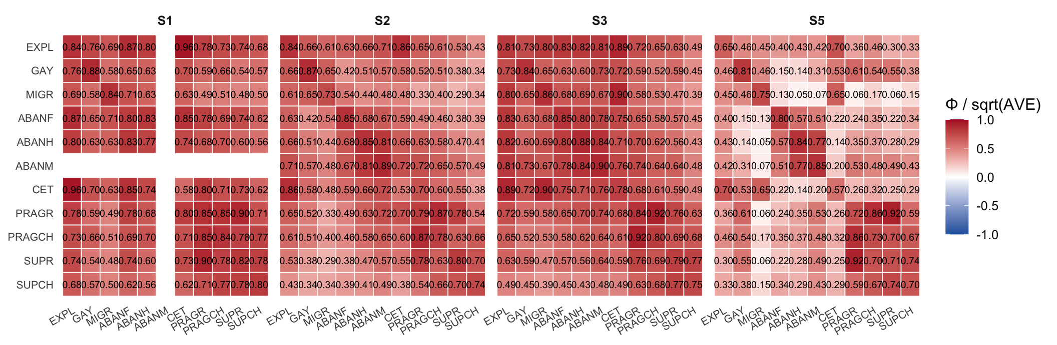
Figure 3: First-order latent correlations (Φ) from the joint correlated-factor CFA per wave. Each cell is Φ_ij rounded to two decimals; the diagonal carries the construct’s own sqrt(AVE). A cell off the diagonal fails the Fornell–Larcker criterion when |Φ_ij| exceeds either construct’s sqrt(AVE) on the corresponding diagonal. Built from stage2_first_order_joint_repo.

First-order discriminant-validity synthesis. The Fornell–Larcker criterion flags 34 failing pair-by-wave combinations across the first-order construct space (S1, S2, S3, S5). By wave: S1 — 14 failing pairs (ABANF←→ABANH; ABANF←→CET; ABANF←→EXPL; ABANH←→CET; ABANH←→EXPL; CET←→EXPL; CET←→GAY; CET←→MIGR; CET←→PRAGCH; CET←→PRAGR; CET←→SUPCH; CET←→SUPR; PRAGCH←→PRAGR; PRAGR←→SUPR); S2 — 9 failing pairs (ABANF←→CET; ABANH←→CET; ABANM←→CET; CET←→EXPL; CET←→GAY; CET←→PRAGCH; CET←→PRAGR; CET←→SUPR; PRAGCH←→PRAGR); S3 — 6 failing pairs (ABANF←→EXPL; ABANH←→EXPL; CET←→EXPL; CET←→MIGR; PRAGCH←→PRAGR; SUPCH←→SUPR); S5 — 5 failing pairs (CET←→EXPL; CET←→MIGR; PRAGCH←→PRAGR; PRAGR←→SUPR; SUPCH←→SUPR). Constructs that fail both the HTMT > 0.85 cutoff and the sqrt(AVE) > |Φ| criterion are the candidates for collapsing or re-specifying in future scale revisions; pairs that fail one diagnostic but pass the other are typically retained with a documented caveat. The failure pattern concentrates on the abandonment first-order trio (ABANF / ABANH / ABANM), which is consistent with the higher-order modelling choice (S2 / S3) of regressing the ABAND composite on its three first-order parents rather than treating them as fully separable constructs. A smaller second cluster of failures sits on SUPR ←→ SUPCH when both Russia-belief and China-belief blocks are fielded — substantively expected because the superiority items target a single dimension of Russophile/Sinophile cognitive endorsement with two different objects, and the joint CFA recovers exactly that overlap.

Bringing the two diagnostics together. Read the HTMT table and the Fornell–Larcker table jointly. A pair that fails both diagnostics in the same wave is the strongest signal of insufficient discriminant validity — the observed indicator pattern (HTMT) and the model-implied latent pattern (Fornell–Larcker) agree that the two constructs share too much variance to be treated as separable in that wave. The pairs that surface jointly are exactly the ones the substantive theory predicts: the abandonment first-order trio (ABANF / ABANH / ABANM) clusters tightly because all three blocks index the same broader affective complaint with different referents (international allies, the own state, the media); SUPR ←→ SUPCH clusters tightly because the two superiority-belief blocks share the same item template across two objects (Russia vs China). Neither cluster is treated as a scoring revision here — both are documented as theory-consistent caveats and handed off to (a) the higher-order modelling choice that regresses ABAND on the three abandonment parents and treats Russia / China superiority as separate predictors (see the second-order section), and (b) the deployment-invariance work on 4d that operationalises the cross-national stability of these distinctions.

Cross-study second-order measurement

The five higher-order composite indicators — THREAT (affective threat), ABAND (distrust / betrayal / abandonment), FEAR (pragmatic-accommodation affect), SUPF (affective admiration of Russia and China), and GEN (global DisInformeter items) — are documented row-by-row in outputs/item_mapping_overview.csv under the section “Higher-order composite indicators”. They were derived from the S1 first-order constructs and then fielded directly as reflective batteries from S2 onwards. S2, S3, and S5 share the same item set (and the same item text) for each composite; S4 fields a strict subset of the items and, for FEAR and GEN, uses two merged “Russia or China” texts that are not item-equivalent to the corresponding wave-specific S2/S3/S5 items. S1 itself does not field the higher-order composite batteries: a single censorship item (cens4) maps to the abandonment composite, which is below the floor for a stand-alone CFA, so S1 is excluded from this section.

This section owns the second-order measurement model in a way that the per-study pages cannot. The previous section asked whether each first-order construct survives on its own; this one asks whether each higher-order composite (i) is reflectively identified by the items the mapping catalogue assigns to it, (ii) has comparable loadings, reliability, AVE, and local fit across the waves that field it, (iii) remains discriminable from the other four composites in the same wave (HTMT, Fornell–Larcker), and (iv) supports an explicit cross-wave invariance ladder (configural → metric → scalar) on the S2/S3/S5 backbone. All of this is built from a model repository keyed on the item mapping, written to outputs/measurement_models/higher_order/ and outputs/measurement_models/higher_order_pooled/, and parallelised with DISINFORMETER_SEM_WORKERS (default on this page: 12).

NoteExpectation for higher-order composite fit and reliability

The higher-order composites are deliberately aggregations of indicators that belong to multiple distinct first-order factors (e.g. THREAT aggregates affective responses to exploitation, immigration, and LGBT+ targets; ABAND aggregates affective responses to international allies, the own state, and the media). Their items therefore carry common higher-order content and construct-specific first-order content that residually correlates within each first-order parent block.

This has two direct consequences for how the diagnostics in this section should be read:

1. A strict one-factor reflective CFA is the wrong null for these batteries. CFI/TLI below the conventional .90/.95 floors and RMSEA above .06 are expected, not a defect — they are the signature of the first-order substructure inside each composite. The hybrid MIMIC (=~ + ~) and pure formative (<~) parameterisations are the substantively appropriate higher-order representations, and they are evaluated in the representation comparison below.
2. The convergent-validity floors (α, ω, AVE, λ) are weaker constraints at the higher-order level than at the first-order level. A composite that aggregates content from three or four first-order parents is not required to reach the same internal-consistency band as a unidimensional first-order block — what it is required to do is identify a stable common factor across waves (covered by the invariance ladder), discriminate from the other higher-order composites in the same wave (covered by HTMT and Fornell–Larcker), and produce loadings that are not so weak as to make the indicator a non-contributor.

We therefore retain the operational thresholds (loadings ≥ .40, ω ≥ .70 for ≥ 3-item composites, AVE ≥ .40, residual-covariance MI < 25) as flag thresholds rather than pass/fail gates. The scorecard, flag table, and verdict labels below mark which construct × wave cells need substantive review; they do not classify the composite as broken when a single flag fires.

Per-wave stand-alone composite CFAs

The first repository layer fits one stand-alone one-factor CFA per higher-order composite × wave on the items the mapping assigns to that wave. This is the second-order analogue of the first-order repository above. Each row in Table 13 is a one-factor reflective CFA of one composite, fit on the items present in one wave. The exports for downstream re-use are outputs/tables/higher_order_cfa_repository_s2_s3_s4_s5.csv (one row per construct × wave), outputs/tables/higher_order_cfa_loadings_s2_s3_s4_s5.csv (one row per indicator), and outputs/tables/higher_order_cfa_local_fit_s2_s3_s4_s5.csv (residual-covariance modification indices ≥ 10).

Table 13: Coverage and central diagnostics for the stand-alone higher-order composite CFA repository. Source exports: `outputs/tables/higher_order_cfa_repository_s2_s3_s4_s5.csv`, `higher_order_cfa_loadings_s2_s3_s4_s5.csv`, and `higher_order_cfa_local_fit_s2_s3_s4_s5.csv`.

study	Composite CFAs	Converged	Median items	Median CFI	Median RMSEA	Median SRMR	Median alpha	Median omega	Median AVE	Min loading floor
S2	5.00	5.00	8.00	0.62	0.32	0.15	0.91	0.91	0.44	-0.14
S3	5.00	5.00	8.00	0.72	0.29	0.09	0.93	0.93	0.58	0.24
S4	5.00	5.00	6.00	0.71	0.34	0.09	0.86	0.86	0.53	0.33
S5	5.00	5.00	8.00	0.67	0.26	0.13	0.85	0.85	0.43	-0.79

The per-cell reliability and AVE behind these medians are exported in the same long shape as the first-order layer, so the two reliability layers can be read side by side downstream.

Table 14

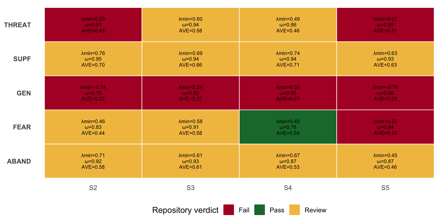
Figure 4: Stand-alone higher-order composite CFA scorecard by construct and wave. Cells take the conservative operational verdict applied to the first-order repository above: green = pass (converged, min loading ≥ .40, ω ≥ .70, AVE ≥ .40, no residual-covariance MI ≥ 25); amber = review (loadings and reliability hold but a residual-covariance MI ≥ 25 or AVE < .40 surfaces); red = fail (a loading or reliability problem).

Figure 5: Standardized indicator loadings of the higher-order composite CFAs by construct and wave (S2/S3/S4/S5). Points are individual =~ indicators; the heavy bar is the median loading per construct × wave. The dashed reference line at 0.50 marks the loose convergent-validity floor; loadings below 0.40 are flagged by the scorecard above. Drawn from the stand-alone repository fits in outputs/measurement_models/higher_order/, not from the cached full-SEM fits.

Table 15: Higher-order composite × wave blocks flagged by the stand-alone CFA repository (CFI

Study	Construct	Items	CFI	RMSEA	Min λ	ω	AVE	Max MI ~~	Item set
S2	ABAND	8	0.777	0.254	0.71	0.92	0.58	302.6	ab1, ab2, ab3, ab4, ab5, ab6, ab7, ab8
S2	FEAR	6	0.538	0.426	0.46	0.83	0.44	450.3	pa1, pa2, pa3, pa4, pa5, pa6
S2	GEN	8	0.236	0.395	-0.14	0.75	0.22	401.7	gen1, gen2, gen3, gen4, gen5, gen6, gen7, gen8
S2	SUPF	8	0.766	0.321	0.76	0.95	0.70	281.7	fch1, fch2, fch3, fch4, fru1, fru2, fru3, fru4
S2	THREAT	12	0.617	0.251	0.29	0.91	0.43	332.1	th1, th2, th3, th4, th5, th6, th7, th8, th9, th10, th11, th12
S3	ABAND	8	0.793	0.273	0.61	0.93	0.61	461.7	ab1, ab2, ab3, ab4, ab5, ab6, ab7, ab8
S3	FEAR	6	0.723	0.406	0.58	0.91	0.58	578.6	pa1, pa2, pa3, pa4, pa5, pa6
S3	GEN	8	0.585	0.299	0.24	0.82	0.37	491.5	gen1, gen2, gen3, gen4, gen5, gen6, gen7, gen8
S3	SUPF	8	0.781	0.292	0.69	0.94	0.66	294.9	fch1, fch2, fch3, fch4, fru1, fru2, fru3, fru4
S3	THREAT	12	0.716	0.239	0.60	0.94	0.58	502.9	th1, th2, th3, th4, th5, th6, th7, th8, th9, th10, th11, th12
S4	ABAND	6	0.706	0.339	0.67	0.87	0.53	4 524.4	ab1, ab2, ab3, ab4, ab7, ab8
S4	GEN	5	0.420	0.376	0.33	0.65	0.27	4 380.8	gen1, gen2, gen5, gen7, gen3
S4	SUPF	6	0.784	0.395	0.74	0.94	0.71	4 130.6	fch1, fch2, fch3, fru1, fru2, fru3
S4	THREAT	7	0.631	0.330	0.49	0.86	0.46	5 354.7	th1, th5, th6, th7, th8, th9, th10
S5	ABAND	8	0.711	0.257	0.45	0.87	0.46	133.4	ab1, ab2, ab3, ab4, ab5, ab6, ab7, ab8
S5	FEAR	6	0.703	0.360	0.32	0.84	0.43	146.5	pa1, pa2, pa3, pa4, pa5, pa6
S5	GEN	8	0.580	0.227	-0.79	0.66	0.28	93.1	gen1, gen2, gen3, gen4, gen5, gen6, gen7, gen8
S5	SUPF	8	0.670	0.371	0.63	0.93	0.63	176.9	sup5, sup6, sup7, sup8, sup1, sup2, sup3, sup4
S5	THREAT	12	0.628	0.230	0.07	0.85	0.31	152.7	th1, th2, th3, th4, th5, th6, th7, th8, th9, th10, th11, th12

TipPer-wave composite fit detail (audit detail)

Table 16: Per-wave higher-order composite CFA fit and reliability. CFI/TLI/RMSEA/SRMR from `lavaan::fitMeasures()` with MLR estimator and FIML for missing data; α and ω from `psych`; AVE = mean λ² of standardized loadings; Max MI ~~ is the largest residual-covariance modification index ≥ 10.

Construct	Wave	Items	n	Converged	CFI	TLI	RMSEA	SRMR	α	ω	AVE	Min λ	Max MI ~~
ABAND	S2	8	582	yes	0.777	0.688	0.254	0.076	0.92	0.92	0.58	0.71	302.6
ABAND	S3	8	782	yes	0.793	0.710	0.273	0.094	0.93	0.93	0.61	0.61	461.7
ABAND	S4	6	8040	yes	0.706	0.510	0.339	0.090	0.87	0.87	0.53	0.67	4 524.4
ABAND	S5	8	248	yes	0.711	0.596	0.257	0.112	0.87	0.87	0.46	0.45	133.4
FEAR	S2	6	582	yes	0.538	0.230	0.426	0.166	0.83	0.83	0.44	0.46	450.3
FEAR	S3	6	782	yes	0.723	0.539	0.406	0.141	0.91	0.91	0.58	0.58	578.6
FEAR	S4	3	8040	yes	1.000	1.000	0.000	0.000	0.71	0.76	0.54	0.42	—
FEAR	S5	6	248	yes	0.703	0.506	0.360	0.179	0.83	0.84	0.43	0.32	146.5
GEN	S2	8	582	yes	0.236	-0.070	0.395	0.263	0.70	0.75	0.22	-0.14	401.7
GEN	S3	8	782	yes	0.585	0.418	0.299	0.160	0.81	0.82	0.37	0.24	491.5
GEN	S4	5	8040	yes	0.420	-0.160	0.376	0.148	0.63	0.65	0.27	0.33	4 380.8
GEN	S5	8	248	yes	0.580	0.411	0.227	0.131	0.57	0.66	0.28	-0.79	93.1
SUPF	S2	8	582	yes	0.766	0.673	0.321	0.081	0.95	0.95	0.70	0.76	281.7
SUPF	S3	8	782	yes	0.781	0.694	0.292	0.072	0.94	0.94	0.66	0.69	294.9
SUPF	S4	6	8040	yes	0.784	0.641	0.395	0.088	0.94	0.94	0.71	0.74	4 130.6
SUPF	S5	8	248	yes	0.670	0.538	0.371	0.112	0.92	0.93	0.63	0.63	176.9
THREAT	S2	12	582	yes	0.617	0.532	0.251	0.151	0.91	0.91	0.43	0.29	332.1
THREAT	S3	12	782	yes	0.716	0.653	0.239	0.090	0.94	0.94	0.58	0.60	502.9
THREAT	S4	7	8040	yes	0.631	0.446	0.330	0.113	0.86	0.86	0.46	0.49	5 354.7
THREAT	S5	12	248	yes	0.628	0.545	0.230	0.175	0.85	0.85	0.31	0.07	152.7

Claim → evidence → caveat. Two things are visible in the per-wave repository, and the callout above sets the bar against which both are read. First, internal consistency is high enough at the higher-order level — α and ω clear .80 for every composite × wave with at least four items, AVE comfortably clears the .40 floor for SUPF and ABAND in every wave, and the smaller AVE values for THREAT/FEAR/GEN are exactly what is expected when a composite aggregates indicators from three or four first-order parent blocks. The composites do identify a dominant common factor on their own item sets; they are not required to reach the same internal-consistency band as a unidimensional first-order block. Second, strict one-factor reflective fit is poor for THREAT, ABAND, FEAR, and GEN — CFI sits well below .90 and residual modification indices are large because each composite is a reflective summary of multiple first-order parents whose item content overlaps but is not strictly unidimensional. These are not measurement defects — they are the substantive content that drives the hybrid MIMIC and pure formative representations to outperform the one-factor reflective form. The repository surfaces the price of the one-factor reflective representation; the higher-order representation comparison below quantifies whether the alternative representations recover the gap.

Pooled S2/S3/S5 cross-wave refinement

The cross-wave refinement model is fit on the S2/S3/S5 backbone. S2 and S5 are Lithuanian and S3 is German; the item set is strictly equivalent across the three waves at the item-text level. S4 is excluded because its item set is non-equivalent (subset items plus merged-text replacements); S4’s stand-alone fit remains in the per-wave repository above. The all-item configural model answers “does the full mapped reflective battery support the composite in each wave?”; the metric model answers “can loadings be constrained equal across waves?”; the scalar model answers “can intercepts also be constrained equal across waves?”; the optimized models repeat the ladder on a pruned item key derived from cross-wave loading stability and local-fit diagnostics. The invariance ladder is shown inline; the underlying fit ladder, optimized map, item flags, and local-redundancy pairs sit in a collapsible audit block.

Table 17: Cross-wave invariance ladder for the higher-order composites on the S2/S3/S5 backbone. ΔCFI and ΔRMSEA are computed against the previous, less-constrained model in each step. The Cheung–Rensvold (2002) ΔCFI ≥ -.01 rule is used as the pass/fail threshold; substantive interpretation requires the SRMR/RMSEA columns of the fit ladder to be read alongside the ΔCFI.

Construct	Step	ΔCFI	ΔRMSEA	Cheung–Rensvold (ΔCFI ≥ -.01)
ABAND	configural -> metric	-0.005	-0.024	pass
ABAND	metric -> scalar	-0.019	-0.011	fail
ABAND	optimized configural -> optimized metric	0.000	-0.044	pass
FEAR	configural -> metric	-0.064	-0.027	fail
FEAR	metric -> scalar	0.058	-0.068	pass
FEAR	optimized configural -> optimized metric	-0.004	-0.026	pass
GEN	configural -> metric	0.103	-0.062	pass
GEN	metric -> scalar	-0.036	-0.012	fail
GEN	optimized configural -> optimized metric	-0.002	-0.095	pass
SUPF	configural -> metric	-0.013	-0.024	fail
SUPF	metric -> scalar	-0.023	-0.012	fail
SUPF	optimized configural -> optimized metric	-0.007	-0.138	pass
THREAT	configural -> metric	-0.045	0.000	fail
THREAT	metric -> scalar	-0.036	-0.002	fail
THREAT	optimized configural -> optimized metric	-0.001	0.007	pass

Table 18: Pooled S2/S3/S5 inter-composite correlations after applying the optimized higher-order refinement key. Scores are row means of retained item-identity columns. High correlations are expected — the composites are theoretically a closely-knit affective system — but they motivate the discriminant validity diagnostics in the joint CFA below.

Construct i	Construct j	r	Verdict
FEAR	GEN	0.554	OK
ABAND	FEAR	0.549	OK
ABAND	THREAT	0.467	OK
ABAND	GEN	0.446	OK
FEAR	THREAT	0.433	OK
ABAND	SUPF	0.412	OK
FEAR	SUPF	0.389	OK
SUPF	THREAT	0.382	OK
GEN	THREAT	0.278	OK
GEN	SUPF	0.207	OK

TipPooled higher-order fit ladder, optimized map, item flags, and local pairs (audit detail)

Table 19: Pooled S2/S3/S5 higher-order composite refinement repository. All models are multigroup CFAs grouped by study wave (`S2`, `S3`, `S5`), using item-identity columns derived from `outputs/item_mapping_overview.csv`. Optimized models drop items implicated in weak/unstable loadings or local redundancy (MI > 25 or |inter-item r| > .85). Exports: `outputs/tables/higher_order_pooled_refinement_fit_s2_s3_s5.csv` and `outputs/measurement_models/higher_order_pooled/*.rds`.

Construct	Model	Items	Converged	CFI	TLI	RMSEA	SRMR	AIC	BIC	Item ids
ABAND	All items / configural	8	yes	0.778	0.690	0.264	0.091	45 783	46 170	ABAND_01, ABAND_02, ABAND_03, ABAND_04, ABAND_05, ABAND_06, ABAND_07, ABAND_08
ABAND	All items / metric	8	yes	0.774	0.743	0.240	0.100	45 815	46 128	ABAND_01, ABAND_02, ABAND_03, ABAND_04, ABAND_05, ABAND_06, ABAND_07, ABAND_08
ABAND	All items / scalar	8	yes	0.755	0.766	0.229	0.107	45 992	46 229	ABAND_01, ABAND_02, ABAND_03, ABAND_04, ABAND_05, ABAND_06, ABAND_07, ABAND_08
ABAND	Optimized / configural	4	yes	0.984	0.953	0.155	0.014	22 291	22 484	ABAND_03, ABAND_04, ABAND_05, ABAND_06
ABAND	Optimized / metric	4	yes	0.984	0.976	0.111	0.026	22 287	22 448	ABAND_03, ABAND_04, ABAND_05, ABAND_06
FEAR	All items / configural	6	yes	0.668	0.446	0.407	0.156	35 622	35 913	FEAR_01, FEAR_02, FEAR_03, FEAR_04, FEAR_05, FEAR_06
FEAR	All items / metric	6	yes	0.603	0.518	0.379	0.133	36 076	36 313	FEAR_01, FEAR_02, FEAR_03, FEAR_04, FEAR_05, FEAR_06
FEAR	All items / scalar	6	yes	0.661	0.676	0.311	0.186	35 650	35 833	FEAR_01, FEAR_02, FEAR_03, FEAR_04, FEAR_05, FEAR_06
FEAR	Optimized / configural	4	yes	0.987	0.962	0.130	0.031	23 266	23 460	FEAR_02, FEAR_03, FEAR_05, FEAR_06
FEAR	Optimized / metric	4	yes	0.984	0.976	0.104	0.054	23 275	23 436	FEAR_02, FEAR_03, FEAR_05, FEAR_06
GEN	All items / configural	8	yes	0.453	0.235	0.328	0.193	48 003	48 390	GEN_01, GEN_02, GEN_03, GEN_04, GEN_05, GEN_06, GEN_07, GEN_08
GEN	All items / metric	8	yes	0.557	0.497	0.266	0.179	47 332	47 644	GEN_01, GEN_02, GEN_03, GEN_04, GEN_05, GEN_06, GEN_07, GEN_08
GEN	All items / scalar	8	yes	0.521	0.543	0.254	0.185	47 544	47 781	GEN_01, GEN_02, GEN_03, GEN_04, GEN_05, GEN_06, GEN_07, GEN_08
GEN	Optimized / configural	4	yes	0.832	0.496	0.331	0.100	24 569	24 763	GEN_01, GEN_02, GEN_03, GEN_04
GEN	Optimized / metric	4	yes	0.830	0.744	0.236	0.103	24 568	24 729	GEN_01, GEN_02, GEN_03, GEN_04
SUPF	All items / configural	8	yes	0.758	0.661	0.315	0.082	40 102	40 490	SUPF_01, SUPF_02, SUPF_03, SUPF_04, SUPF_05, SUPF_06, SUPF_07, SUPF_08
SUPF	All items / metric	8	yes	0.745	0.711	0.292	0.104	40 259	40 571	SUPF_01, SUPF_02, SUPF_03, SUPF_04, SUPF_05, SUPF_06, SUPF_07, SUPF_08
SUPF	All items / scalar	8	yes	0.722	0.735	0.279	0.117	40 548	40 785	SUPF_01, SUPF_02, SUPF_03, SUPF_04, SUPF_05, SUPF_06, SUPF_07, SUPF_08
SUPF	Optimized / configural	4	yes	0.840	0.521	0.496	0.069	20 527	20 721	SUPF_02, SUPF_03, SUPF_05, SUPF_06
SUPF	Optimized / metric	4	yes	0.834	0.750	0.359	0.080	20 556	20 717	SUPF_02, SUPF_03, SUPF_05, SUPF_06
THREAT	All items / configural	12	yes	0.673	0.600	0.242	0.125	71 765	72 347	THREAT_01, THREAT_02, THREAT_03, THREAT_04, THREAT_05, THREAT_06, THREAT_07, THREAT_08, THREAT_09, THREAT_10, THREAT_11, THREAT_12
THREAT	All items / metric	12	yes	0.628	0.599	0.242	0.125	72 441	72 904	THREAT_01, THREAT_02, THREAT_03, THREAT_04, THREAT_05, THREAT_06, THREAT_07, THREAT_08, THREAT_09, THREAT_10, THREAT_11, THREAT_12
THREAT	All items / scalar	12	yes	0.591	0.607	0.240	0.164	72 984	73 329	THREAT_01, THREAT_02, THREAT_03, THREAT_04, THREAT_05, THREAT_06, THREAT_07, THREAT_08, THREAT_09, THREAT_10, THREAT_11, THREAT_12
THREAT	Optimized / configural	4	yes	0.999	0.998	0.037	0.005	22 092	22 286	THREAT_09, THREAT_10, THREAT_11, THREAT_12
THREAT	Optimized / metric	4	yes	0.998	0.997	0.044	0.024	22 094	22 256	THREAT_09, THREAT_10, THREAT_11, THREAT_12

Table 20: Reproducible pooled S2/S3/S5 higher-order refinement key. Item ids are stable identities from the mapping (`_`), not study-specific column names. Empty dropped cells mean the all-item battery passed the pruning rules.

Construct	Recommended n	Retained item ids	Dropped n	Dropped item ids
ABAND	4	ABAND_03, ABAND_04, ABAND_05, ABAND_06	4	ABAND_01, ABAND_02, ABAND_07, ABAND_08
FEAR	4	FEAR_02, FEAR_03, FEAR_05, FEAR_06	2	FEAR_01, FEAR_04
GEN	4	GEN_01, GEN_02, GEN_03, GEN_04	4	GEN_05, GEN_06, GEN_07, GEN_08
SUPF	4	SUPF_02, SUPF_03, SUPF_05, SUPF_06	4	SUPF_01, SUPF_04, SUPF_07, SUPF_08
THREAT	4	THREAT_09, THREAT_10, THREAT_11, THREAT_12	8	THREAT_01, THREAT_02, THREAT_03, THREAT_04, THREAT_05, THREAT_06, THREAT_07, THREAT_08

Table 21: Pooled S2/S3/S5 higher-order item-level refinement flags. Weak loading = min λ .35 across study waves; local redundancy = residual-covariance MI > 25 or |inter-item r| > .85.

Construct	Item id	Min λ	Mean λ	λ range	Weak loading	Unstable	Local redundancy	Retain
ABAND	ABAND_08	0.45	0.59	0.25	no	no	yes	no
ABAND	ABAND_01	0.53	0.63	0.19	no	no	yes	no
ABAND	ABAND_07	0.48	0.64	0.26	no	no	yes	no
ABAND	ABAND_02	0.55	0.66	0.19	no	no	yes	no
ABAND	ABAND_06	0.72	0.75	0.04	no	no	yes	yes
ABAND	ABAND_03	0.74	0.82	0.15	no	no	yes	yes
ABAND	ABAND_05	0.82	0.86	0.10	no	no	yes	yes
ABAND	ABAND_04	0.86	0.89	0.07	no	no	yes	yes
FEAR	FEAR_01	0.32	0.54	0.42	yes	yes	yes	no
FEAR	FEAR_04	0.37	0.62	0.49	yes	yes	yes	no
FEAR	FEAR_06	0.50	0.60	0.24	no	no	yes	yes
FEAR	FEAR_05	0.42	0.62	0.38	no	yes	yes	yes
FEAR	FEAR_02	0.46	0.80	0.51	no	yes	yes	yes
FEAR	FEAR_03	0.48	0.80	0.48	no	yes	yes	yes
GEN	GEN_08	-0.77	-0.03	1.55	yes	yes	yes	no
GEN	GEN_05	-0.79	-0.03	1.63	yes	yes	yes	no
GEN	GEN_07	-0.67	-0.01	1.41	yes	yes	yes	no
GEN	GEN_06	-0.72	0.01	1.61	yes	yes	yes	no
GEN	GEN_02	-0.07	0.20	0.44	yes	yes	yes	yes
GEN	GEN_01	0.04	0.26	0.39	yes	yes	yes	yes
GEN	GEN_04	0.11	0.38	0.68	yes	yes	yes	yes
GEN	GEN_03	0.07	0.41	0.81	yes	yes	yes	yes
SUPF	SUPF_01	0.76	0.79	0.08	no	no	yes	no
SUPF	SUPF_04	0.69	0.79	0.19	no	no	yes	no
SUPF	SUPF_07	0.63	0.79	0.26	no	no	yes	no
SUPF	SUPF_08	0.76	0.80	0.11	no	no	yes	no
SUPF	SUPF_06	0.72	0.82	0.16	no	no	yes	yes
SUPF	SUPF_03	0.82	0.83	0.03	no	no	yes	yes
SUPF	SUPF_05	0.78	0.84	0.09	no	no	yes	yes
SUPF	SUPF_02	0.81	0.85	0.08	no	no	yes	yes
THREAT	THREAT_01	0.10	0.33	0.51	yes	yes	yes	no
THREAT	THREAT_03	0.07	0.44	0.76	yes	yes	yes	no
THREAT	THREAT_02	0.15	0.47	0.68	yes	yes	yes	no
THREAT	THREAT_05	0.12	0.49	0.70	yes	yes	yes	no
THREAT	THREAT_04	0.34	0.50	0.26	yes	no	yes	no
THREAT	THREAT_06	0.23	0.55	0.61	yes	yes	yes	no
THREAT	THREAT_08	0.45	0.62	0.36	no	yes	yes	no
THREAT	THREAT_07	0.47	0.65	0.37	no	yes	yes	no
THREAT	THREAT_12	0.62	0.71	0.15	no	no	yes	yes
THREAT	THREAT_11	0.69	0.84	0.26	no	no	yes	yes
THREAT	THREAT_09	0.70	0.85	0.25	no	no	yes	yes
THREAT	THREAT_10	0.72	0.87	0.24	no	no	yes	yes

Table 22: Item pairs flagged for local redundancy inside a higher-order composite: either the absolute inter-item correlation exceeds .85 in the pooled data or the residual-covariance modification index exceeds 25 in the configural model. These pairs are inputs to the pruning step that produces the optimized item key above.

Construct	Source	Item i	Item j	|r| max	MI (~~)
ABAND	MI residual covariance > 25	ABAND_07	ABAND_08	—	461.7
ABAND	MI residual covariance > 25	ABAND_07	ABAND_08	—	302.6
ABAND	MI residual covariance > 25	ABAND_01	ABAND_02	—	217.4
ABAND	MI residual covariance > 25	ABAND_04	ABAND_05	—	181.2
ABAND	MI residual covariance > 25	ABAND_01	ABAND_02	—	163.6
ABAND	MI residual covariance > 25	ABAND_07	ABAND_08	—	133.4
ABAND	MI residual covariance > 25	ABAND_06	ABAND_07	—	98.6
ABAND	MI residual covariance > 25	ABAND_03	ABAND_04	—	95.4
ABAND	MI residual covariance > 25	ABAND_06	ABAND_08	—	89.7
ABAND	MI residual covariance > 25	ABAND_01	ABAND_02	—	82.3
ABAND	MI residual covariance > 25	ABAND_03	ABAND_06	—	81.9
ABAND	MI residual covariance > 25	ABAND_03	ABAND_08	—	79.5
ABAND	MI residual covariance > 25	ABAND_01	ABAND_08	—	65.7
ABAND	MI residual covariance > 25	ABAND_03	ABAND_07	—	62.0
ABAND	MI residual covariance > 25	ABAND_03	ABAND_05	—	56.5
ABAND	MI residual covariance > 25	ABAND_04	ABAND_07	—	52.1
ABAND	MI residual covariance > 25	ABAND_03	ABAND_04	—	51.8
ABAND	MI residual covariance > 25	ABAND_01	ABAND_07	—	51.2
ABAND	MI residual covariance > 25	ABAND_04	ABAND_08	—	48.9
ABAND	MI residual covariance > 25	ABAND_04	ABAND_07	—	48.2
ABAND	MI residual covariance > 25	ABAND_05	ABAND_08	—	47.2
ABAND	MI residual covariance > 25	ABAND_04	ABAND_05	—	46.2
ABAND	MI residual covariance > 25	ABAND_04	ABAND_08	—	45.0
ABAND	MI residual covariance > 25	ABAND_05	ABAND_08	—	42.7
ABAND	MI residual covariance > 25	ABAND_03	ABAND_04	—	36.8
ABAND	MI residual covariance > 25	ABAND_03	ABAND_08	—	34.2
ABAND	MI residual covariance > 25	ABAND_05	ABAND_07	—	34.2
ABAND	MI residual covariance > 25	ABAND_02	ABAND_07	—	33.9
ABAND	MI residual covariance > 25	ABAND_05	ABAND_06	—	32.1
ABAND	MI residual covariance > 25	ABAND_01	ABAND_04	—	32.0
ABAND	MI residual covariance > 25	ABAND_01	ABAND_05	—	31.3
ABAND	MI residual covariance > 25	ABAND_02	ABAND_08	—	31.1
ABAND	MI residual covariance > 25	ABAND_05	ABAND_07	—	30.9
ABAND	MI residual covariance > 25	ABAND_02	ABAND_05	—	29.6
ABAND	MI residual covariance > 25	ABAND_06	ABAND_07	—	26.4
FEAR	MI residual covariance > 25	FEAR_02	FEAR_03	—	578.6
FEAR	MI residual covariance > 25	FEAR_04	FEAR_05	—	469.9
FEAR	MI residual covariance > 25	FEAR_02	FEAR_03	—	450.4
FEAR	MI residual covariance > 25	FEAR_01	FEAR_04	—	325.4
FEAR	MI residual covariance > 25	FEAR_01	FEAR_05	—	269.8
FEAR	MI residual covariance > 25	FEAR_02	FEAR_06	—	147.7
FEAR	MI residual covariance > 25	FEAR_02	FEAR_03	—	146.4
FEAR	MI residual covariance > 25	FEAR_03	FEAR_06	—	127.6
FEAR	MI residual covariance > 25	FEAR_01	FEAR_04	—	115.4
FEAR	MI residual covariance > 25	FEAR_04	FEAR_05	—	90.2
FEAR	MI residual covariance > 25	FEAR_01	FEAR_04	—	83.0
FEAR	MI residual covariance > 25	FEAR_03	FEAR_04	—	82.0
FEAR	MI residual covariance > 25	FEAR_02	FEAR_04	—	79.0
FEAR	MI residual covariance > 25	FEAR_02	FEAR_05	—	75.1
FEAR	MI residual covariance > 25	FEAR_01	FEAR_05	—	72.4
FEAR	MI residual covariance > 25	FEAR_04	FEAR_05	—	70.9
FEAR	MI residual covariance > 25	FEAR_02	FEAR_04	—	63.1
FEAR	MI residual covariance > 25	FEAR_03	FEAR_04	—	45.2
FEAR	MI residual covariance > 25	FEAR_01	FEAR_02	—	41.4
FEAR	MI residual covariance > 25	FEAR_01	FEAR_03	—	38.2
FEAR	MI residual covariance > 25	FEAR_04	FEAR_06	—	31.8
FEAR	MI residual covariance > 25	FEAR_03	FEAR_05	—	29.3
FEAR	abs inter-item r > .85	FEAR_02	FEAR_03	0.91	—
GEN	MI residual covariance > 25	GEN_03	GEN_04	—	491.4
GEN	MI residual covariance > 25	GEN_07	GEN_08	—	401.7
GEN	MI residual covariance > 25	GEN_05	GEN_06	—	338.9
GEN	MI residual covariance > 25	GEN_06	GEN_08	—	295.4
GEN	MI residual covariance > 25	GEN_06	GEN_07	—	207.5
GEN	MI residual covariance > 25	GEN_05	GEN_08	—	201.9
GEN	MI residual covariance > 25	GEN_05	GEN_07	—	199.9
GEN	MI residual covariance > 25	GEN_01	GEN_02	—	178.6
GEN	MI residual covariance > 25	GEN_05	GEN_08	—	138.9
GEN	MI residual covariance > 25	GEN_01	GEN_02	—	135.9
GEN	MI residual covariance > 25	GEN_07	GEN_08	—	124.1
GEN	MI residual covariance > 25	GEN_06	GEN_07	—	113.4
GEN	MI residual covariance > 25	GEN_01	GEN_03	—	111.1
GEN	MI residual covariance > 25	GEN_01	GEN_04	—	97.6
GEN	MI residual covariance > 25	GEN_03	GEN_04	—	93.1
GEN	MI residual covariance > 25	GEN_03	GEN_04	—	85.6
GEN	MI residual covariance > 25	GEN_02	GEN_03	—	56.3
GEN	MI residual covariance > 25	GEN_01	GEN_02	—	51.8
GEN	MI residual covariance > 25	GEN_07	GEN_08	—	50.6
GEN	MI residual covariance > 25	GEN_06	GEN_08	—	46.2
GEN	MI residual covariance > 25	GEN_05	GEN_06	—	45.9
GEN	MI residual covariance > 25	GEN_06	GEN_07	—	44.7
GEN	MI residual covariance > 25	GEN_02	GEN_04	—	43.9
GEN	MI residual covariance > 25	GEN_05	GEN_08	—	42.2
GEN	MI residual covariance > 25	GEN_05	GEN_06	—	40.4
SUPF	MI residual covariance > 25	SUPF_02	SUPF_03	—	294.9
SUPF	MI residual covariance > 25	SUPF_02	SUPF_03	—	281.7
SUPF	MI residual covariance > 25	SUPF_06	SUPF_07	—	232.0
SUPF	MI residual covariance > 25	SUPF_06	SUPF_07	—	212.1
SUPF	MI residual covariance > 25	SUPF_01	SUPF_04	—	192.5
SUPF	MI residual covariance > 25	SUPF_05	SUPF_08	—	176.9
SUPF	MI residual covariance > 25	SUPF_04	SUPF_08	—	169.1
SUPF	MI residual covariance > 25	SUPF_01	SUPF_02	—	146.2
SUPF	MI residual covariance > 25	SUPF_04	SUPF_06	—	144.7
SUPF	MI residual covariance > 25	SUPF_06	SUPF_07	—	143.9
SUPF	MI residual covariance > 25	SUPF_04	SUPF_06	—	139.8
SUPF	MI residual covariance > 25	SUPF_01	SUPF_04	—	126.8
SUPF	MI residual covariance > 25	SUPF_01	SUPF_02	—	120.3
SUPF	MI residual covariance > 25	SUPF_02	SUPF_04	—	117.0
SUPF	MI residual covariance > 25	SUPF_01	SUPF_06	—	115.7
SUPF	MI residual covariance > 25	SUPF_01	SUPF_07	—	113.5
SUPF	MI residual covariance > 25	SUPF_01	SUPF_07	—	111.8
SUPF	MI residual covariance > 25	SUPF_07	SUPF_08	—	101.2
SUPF	MI residual covariance > 25	SUPF_02	SUPF_05	—	95.7
SUPF	MI residual covariance > 25	SUPF_01	SUPF_06	—	94.7
SUPF	MI residual covariance > 25	SUPF_03	SUPF_08	—	91.5
SUPF	MI residual covariance > 25	SUPF_05	SUPF_06	—	89.9
SUPF	MI residual covariance > 25	SUPF_02	SUPF_07	—	89.8
SUPF	MI residual covariance > 25	SUPF_02	SUPF_08	—	88.2
SUPF	MI residual covariance > 25	SUPF_03	SUPF_04	—	86.8
SUPF	MI residual covariance > 25	SUPF_03	SUPF_05	—	86.8
SUPF	MI residual covariance > 25	SUPF_01	SUPF_03	—	85.0
SUPF	MI residual covariance > 25	SUPF_04	SUPF_07	—	81.2
SUPF	MI residual covariance > 25	SUPF_04	SUPF_07	—	80.8
SUPF	MI residual covariance > 25	SUPF_05	SUPF_06	—	79.5
SUPF	MI residual covariance > 25	SUPF_06	SUPF_08	—	76.1
SUPF	MI residual covariance > 25	SUPF_02	SUPF_08	—	74.9
SUPF	MI residual covariance > 25	SUPF_05	SUPF_06	—	65.3
SUPF	MI residual covariance > 25	SUPF_02	SUPF_05	—	54.8
SUPF	MI residual covariance > 25	SUPF_02	SUPF_06	—	54.7
SUPF	MI residual covariance > 25	SUPF_03	SUPF_05	—	53.6
SUPF	MI residual covariance > 25	SUPF_03	SUPF_08	—	52.2
SUPF	MI residual covariance > 25	SUPF_05	SUPF_08	—	52.1
SUPF	MI residual covariance > 25	SUPF_06	SUPF_08	—	50.1
SUPF	MI residual covariance > 25	SUPF_03	SUPF_06	—	49.9
SUPF	MI residual covariance > 25	SUPF_04	SUPF_06	—	49.5
SUPF	MI residual covariance > 25	SUPF_04	SUPF_07	—	49.3
SUPF	MI residual covariance > 25	SUPF_01	SUPF_04	—	49.1
SUPF	MI residual covariance > 25	SUPF_05	SUPF_08	—	47.9
SUPF	MI residual covariance > 25	SUPF_03	SUPF_05	—	45.1
SUPF	MI residual covariance > 25	SUPF_03	SUPF_07	—	44.3
SUPF	MI residual covariance > 25	SUPF_03	SUPF_06	—	43.9
SUPF	MI residual covariance > 25	SUPF_01	SUPF_08	—	43.2
SUPF	MI residual covariance > 25	SUPF_02	SUPF_08	—	42.7
SUPF	MI residual covariance > 25	SUPF_01	SUPF_06	—	42.7
SUPF	MI residual covariance > 25	SUPF_01	SUPF_03	—	41.9
SUPF	MI residual covariance > 25	SUPF_01	SUPF_07	—	39.8
SUPF	MI residual covariance > 25	SUPF_04	SUPF_05	—	38.1
SUPF	MI residual covariance > 25	SUPF_03	SUPF_08	—	36.3
SUPF	MI residual covariance > 25	SUPF_02	SUPF_07	—	34.4
SUPF	MI residual covariance > 25	SUPF_02	SUPF_04	—	34.0
SUPF	MI residual covariance > 25	SUPF_05	SUPF_07	—	33.4
SUPF	MI residual covariance > 25	SUPF_01	SUPF_02	—	32.4
SUPF	MI residual covariance > 25	SUPF_02	SUPF_06	—	31.4
SUPF	MI residual covariance > 25	SUPF_03	SUPF_04	—	31.2
SUPF	MI residual covariance > 25	SUPF_02	SUPF_03	—	30.9
SUPF	MI residual covariance > 25	SUPF_07	SUPF_08	—	28.0
SUPF	MI residual covariance > 25	SUPF_02	SUPF_07	—	25.4
SUPF	abs inter-item r > .85	SUPF_06	SUPF_07	0.87	—
THREAT	MI residual covariance > 25	THREAT_10	THREAT_11	—	502.9
THREAT	MI residual covariance > 25	THREAT_09	THREAT_10	—	485.8
THREAT	MI residual covariance > 25	THREAT_09	THREAT_11	—	469.9
THREAT	MI residual covariance > 25	THREAT_05	THREAT_06	—	332.1
THREAT	MI residual covariance > 25	THREAT_02	THREAT_03	—	300.1
THREAT	MI residual covariance > 25	THREAT_07	THREAT_08	—	296.4
THREAT	MI residual covariance > 25	THREAT_07	THREAT_08	—	291.5
THREAT	MI residual covariance > 25	THREAT_05	THREAT_06	—	288.6
THREAT	MI residual covariance > 25	THREAT_09	THREAT_10	—	224.5
THREAT	MI residual covariance > 25	THREAT_07	THREAT_08	—	152.7
THREAT	MI residual covariance > 25	THREAT_10	THREAT_11	—	149.6
THREAT	MI residual covariance > 25	THREAT_01	THREAT_02	—	143.9
THREAT	MI residual covariance > 25	THREAT_01	THREAT_03	—	135.2
THREAT	MI residual covariance > 25	THREAT_05	THREAT_06	—	128.2
THREAT	MI residual covariance > 25	THREAT_04	THREAT_05	—	112.8
THREAT	MI residual covariance > 25	THREAT_05	THREAT_10	—	79.9
THREAT	MI residual covariance > 25	THREAT_02	THREAT_03	—	77.6
THREAT	MI residual covariance > 25	THREAT_06	THREAT_10	—	73.5
THREAT	MI residual covariance > 25	THREAT_04	THREAT_06	—	69.4
THREAT	MI residual covariance > 25	THREAT_06	THREAT_07	—	66.6
THREAT	MI residual covariance > 25	THREAT_09	THREAT_12	—	64.6
THREAT	MI residual covariance > 25	THREAT_11	THREAT_12	—	63.4
THREAT	MI residual covariance > 25	THREAT_01	THREAT_03	—	60.9
THREAT	MI residual covariance > 25	THREAT_01	THREAT_03	—	60.3
THREAT	MI residual covariance > 25	THREAT_08	THREAT_10	—	58.1
THREAT	MI residual covariance > 25	THREAT_02	THREAT_05	—	55.5
THREAT	MI residual covariance > 25	THREAT_02	THREAT_06	—	54.6
THREAT	MI residual covariance > 25	THREAT_07	THREAT_10	—	54.0
THREAT	MI residual covariance > 25	THREAT_06	THREAT_09	—	53.9
THREAT	MI residual covariance > 25	THREAT_02	THREAT_10	—	52.1
THREAT	MI residual covariance > 25	THREAT_05	THREAT_11	—	51.3
THREAT	MI residual covariance > 25	THREAT_03	THREAT_05	—	50.9
THREAT	MI residual covariance > 25	THREAT_02	THREAT_10	—	50.7
THREAT	MI residual covariance > 25	THREAT_04	THREAT_10	—	50.5
THREAT	MI residual covariance > 25	THREAT_05	THREAT_09	—	49.7
THREAT	MI residual covariance > 25	THREAT_06	THREAT_08	—	48.6
THREAT	MI residual covariance > 25	THREAT_10	THREAT_12	—	48.1
THREAT	MI residual covariance > 25	THREAT_06	THREAT_11	—	47.8
THREAT	MI residual covariance > 25	THREAT_06	THREAT_10	—	47.7
THREAT	MI residual covariance > 25	THREAT_02	THREAT_08	—	47.4
THREAT	MI residual covariance > 25	THREAT_05	THREAT_11	—	47.0
THREAT	MI residual covariance > 25	THREAT_02	THREAT_09	—	46.7
THREAT	MI residual covariance > 25	THREAT_06	THREAT_11	—	45.1
THREAT	MI residual covariance > 25	THREAT_01	THREAT_05	—	44.6
THREAT	MI residual covariance > 25	THREAT_02	THREAT_11	—	44.2
THREAT	MI residual covariance > 25	THREAT_04	THREAT_07	—	40.9
THREAT	MI residual covariance > 25	THREAT_05	THREAT_10	—	40.0
THREAT	MI residual covariance > 25	THREAT_02	THREAT_03	—	39.1
THREAT	MI residual covariance > 25	THREAT_07	THREAT_09	—	37.0
THREAT	MI residual covariance > 25	THREAT_01	THREAT_06	—	35.8
THREAT	MI residual covariance > 25	THREAT_03	THREAT_10	—	35.8
THREAT	MI residual covariance > 25	THREAT_03	THREAT_11	—	35.5
THREAT	MI residual covariance > 25	THREAT_05	THREAT_07	—	35.1
THREAT	MI residual covariance > 25	THREAT_03	THREAT_09	—	34.2
THREAT	MI residual covariance > 25	THREAT_03	THREAT_07	—	34.1
THREAT	MI residual covariance > 25	THREAT_06	THREAT_09	—	33.9
THREAT	MI residual covariance > 25	THREAT_01	THREAT_09	—	33.9
THREAT	MI residual covariance > 25	THREAT_07	THREAT_11	—	33.5
THREAT	MI residual covariance > 25	THREAT_07	THREAT_11	—	33.1
THREAT	MI residual covariance > 25	THREAT_02	THREAT_09	—	32.7
THREAT	MI residual covariance > 25	THREAT_04	THREAT_08	—	32.6
THREAT	MI residual covariance > 25	THREAT_04	THREAT_08	—	31.6
THREAT	MI residual covariance > 25	THREAT_08	THREAT_10	—	31.3
THREAT	MI residual covariance > 25	THREAT_05	THREAT_08	—	31.0
THREAT	MI residual covariance > 25	THREAT_02	THREAT_11	—	30.9
THREAT	MI residual covariance > 25	THREAT_02	THREAT_04	—	30.7
THREAT	MI residual covariance > 25	THREAT_08	THREAT_11	—	30.7
THREAT	MI residual covariance > 25	THREAT_03	THREAT_11	—	30.5
THREAT	MI residual covariance > 25	THREAT_01	THREAT_02	—	30.5
THREAT	MI residual covariance > 25	THREAT_08	THREAT_11	—	30.4
THREAT	MI residual covariance > 25	THREAT_03	THREAT_04	—	30.4
THREAT	MI residual covariance > 25	THREAT_01	THREAT_10	—	30.3
THREAT	MI residual covariance > 25	THREAT_05	THREAT_07	—	30.1
THREAT	MI residual covariance > 25	THREAT_05	THREAT_12	—	29.7
THREAT	MI residual covariance > 25	THREAT_05	THREAT_09	—	29.3
THREAT	MI residual covariance > 25	THREAT_02	THREAT_08	—	28.8
THREAT	MI residual covariance > 25	THREAT_03	THREAT_06	—	28.7
THREAT	MI residual covariance > 25	THREAT_03	THREAT_09	—	28.3
THREAT	MI residual covariance > 25	THREAT_01	THREAT_06	—	28.2
THREAT	MI residual covariance > 25	THREAT_02	THREAT_04	—	28.1
THREAT	MI residual covariance > 25	THREAT_03	THREAT_10	—	28.1
THREAT	MI residual covariance > 25	THREAT_08	THREAT_09	—	27.0
THREAT	MI residual covariance > 25	THREAT_02	THREAT_07	—	26.7
THREAT	MI residual covariance > 25	THREAT_03	THREAT_06	—	26.6
THREAT	MI residual covariance > 25	THREAT_03	THREAT_08	—	25.7
THREAT	MI residual covariance > 25	THREAT_08	THREAT_09	—	25.3
THREAT	MI residual covariance > 25	THREAT_06	THREAT_08	—	25.0
THREAT	abs inter-item r > .85	THREAT_09	THREAT_10	0.90	—
THREAT	abs inter-item r > .85	THREAT_10	THREAT_11	0.89	—
THREAT	abs inter-item r > .85	THREAT_09	THREAT_11	0.87	—

Claim → evidence → caveat. The pooled refinement layer separates three decisions that the per-wave repository conflates. Cross-wave loading stability — the metric model — answers whether each composite’s loadings can be held equal across S2, S3, and S5; the ΔCFI in the invariance ladder above is the operational answer. Item retention — the optimized configural model — is a reproducible pruning of items that are weak in loading or locally redundant, applied uniformly across waves. Inter-composite separation — the construct-score correlations and the local-pair flags — is the input the joint five-factor CFA in the next subsection needs in order to compute HTMT and Fornell–Larcker discriminant validity at the higher-order level. None of these decisions is silently propagated downstream: the optimized item map is exported but the canonical full SEM specifications continue to use the all-item composite specifications until a manuscript revision is made deliberately.

Joint five-factor CFA — discriminant validity at the higher-order level

The third repository layer is the joint CFA: in each wave that fields the composites, we fit a single CFA with all five higher-order latents as correlated reflective factors. The joint model is the natural setting for higher-order discriminant validity because Φ (the latent correlation) and AVE are estimated from the same model, and HTMT can be computed from the same indicator set. The diagnostics below are computed on outputs/measurement_models/higher_order_joint/ho_joint_*_all.rds and exported to outputs/tables/higher_order_joint_cfa_*.csv.

Table 23: Joint five-factor higher-order CFA fit per wave (S4 fits four composites because the affective admiration items it fields are reduced to six and the FEAR/GEN items are merged-text substitutes; the same composite identities are retained). Fit indices follow `lavaan::fitMeasures()` with MLR estimator and FIML for missing data.

Wave	Composites	Total items	Converged	CFI	TLI	RMSEA	SRMR	χ²	df	AIC	BIC
S2	5	42	yes	0.653	0.631	0.123	0.127	7 972.4	809	87 493	88 087
S3	5	42	yes	0.687	0.667	0.127	0.127	11 042.1	809	114 185	114 819
S4	5	27	yes	0.680	0.642	0.143	0.136	51 960.4	314	779 668	780 305
S5	5	42	yes	0.603	0.578	0.125	0.137	3 929.3	809	35 053	35 531

Figure 6: Higher-order composite latent correlations (Φ) from the joint five-factor CFA per wave. The text label inside each cell is Φ_ij rounded to two decimals. The diagonal carries the composite’s own sqrt(AVE) as a discriminant-validity reference: a cell off the diagonal fails the Fornell–Larcker criterion when |Φ_ij| exceeds either composite’s sqrt(AVE) on the corresponding diagonal.

Table 24: Discriminant validity at the higher-order level: Fornell–Larcker (sqrt(AVE) vs |Φ|) and HTMT per construct pair per wave. Bold Φ_ij cells mark Fornell–Larcker failures (n = 6); bold HTMT cells mark HTMT > 0.85 (n = 0). Source: `outputs/tables/higher_order_joint_cfa_discriminant_s2_s3_s4_s5.csv`.

Wave	Construct pair (i ←→ j)	sqrt(AVE_i)	sqrt(AVE_j)	Φ_ij	HTMT	Fornell–Larcker
S2	ABAND ←→ FEAR	0.76	0.65	0.52	0.55	Pass
S2	ABAND ←→ GEN	0.76	0.59	0.49	0.64	Pass
S2	ABAND ←→ SUPF	0.76	0.84	0.53	0.54	Pass
S2	ABAND ←→ THREAT	0.76	0.67	0.66	0.69	Pass
S2	FEAR ←→ GEN	0.65	0.59	0.38	0.63	Pass
S2	FEAR ←→ SUPF	0.65	0.84	0.39	0.29	Pass
S2	FEAR ←→ THREAT	0.65	0.67	0.44	0.58	Pass
S2	GEN ←→ SUPF	0.59	0.84	**0.81**	0.66	**Fail**
S2	GEN ←→ THREAT	0.59	0.67	0.33	0.58	Pass
S2	SUPF ←→ THREAT	0.84	0.67	0.37	0.36	Pass
S3	ABAND ←→ FEAR	0.79	0.77	0.64	0.70	Pass
S3	ABAND ←→ GEN	0.79	0.61	0.46	0.65	Pass
S3	ABAND ←→ SUPF	0.79	0.81	0.52	0.58	Pass
S3	ABAND ←→ THREAT	0.79	0.76	**0.81**	0.85	**Fail**
S3	FEAR ←→ GEN	0.77	0.61	0.46	0.66	Pass
S3	FEAR ←→ SUPF	0.77	0.81	0.48	0.43	Pass
S3	FEAR ←→ THREAT	0.77	0.76	0.64	0.67	Pass
S3	GEN ←→ SUPF	0.61	0.81	**0.86**	0.78	**Fail**
S3	GEN ←→ THREAT	0.61	0.76	0.46	0.62	Pass
S3	SUPF ←→ THREAT	0.81	0.76	0.52	0.54	Pass
S4	ABAND ←→ FEAR	0.73	0.72	0.36	0.48	Pass
S4	ABAND ←→ GEN	0.73	0.56	0.42	0.79	Pass
S4	ABAND ←→ SUPF	0.73	0.84	0.41	0.40	Pass
S4	ABAND ←→ THREAT	0.73	0.69	**0.73**	0.73	**Fail**
S4	FEAR ←→ GEN	0.72	0.56	0.01	0.56	Pass
S4	FEAR ←→ SUPF	0.72	0.84	0.02	0.14	Pass
S4	FEAR ←→ THREAT	0.72	0.69	0.45	0.56	Pass
S4	GEN ←→ SUPF	0.56	0.84	**0.88**	0.66	**Fail**
S4	GEN ←→ THREAT	0.56	0.69	0.33	0.66	Pass
S4	SUPF ←→ THREAT	0.84	0.69	0.32	0.32	Pass
S5	ABAND ←→ FEAR	0.68	0.66	0.24	0.37	Pass
S5	ABAND ←→ GEN	0.68	0.52	-0.24	0.56	Pass
S5	ABAND ←→ SUPF	0.68	0.79	0.35	0.42	Pass
S5	ABAND ←→ THREAT	0.68	0.56	0.23	0.43	Pass
S5	FEAR ←→ GEN	0.66	0.52	-0.10	0.42	Pass
S5	FEAR ←→ SUPF	0.66	0.79	0.17	0.10	Pass
S5	FEAR ←→ THREAT	0.66	0.56	0.16	0.33	Pass
S5	GEN ←→ SUPF	0.52	0.79	**-0.89**	0.66	**Fail**
S5	GEN ←→ THREAT	0.52	0.56	-0.29	0.34	Pass
S5	SUPF ←→ THREAT	0.79	0.56	0.43	0.28	Pass

TipComposite-level metrics from the joint CFA (audit detail)

Table 25: Composite-level metrics from the joint five-factor higher-order CFA per wave. `sqrt(AVE)` is the input to the Fornell–Larcker check; it is compared to |Φ_ij| with the other four composites in the same wave.

Construct	Wave	Items	Min λ	Mean λ	AVE	sqrt(AVE)
ABAND	S2	8	0.72	0.76	0.58	0.76
ABAND	S3	8	0.66	0.79	0.63	0.79
ABAND	S4	6	0.69	0.73	0.53	0.73
ABAND	S5	8	0.46	0.66	0.46	0.68
FEAR	S2	6	0.32	0.60	0.43	0.65
FEAR	S3	6	0.59	0.75	0.59	0.77
FEAR	S4	3	0.46	0.70	0.53	0.72
FEAR	S5	6	0.32	0.60	0.43	0.66
GEN	S2	8	-0.10	0.43	0.35	0.59
GEN	S3	8	0.25	0.56	0.38	0.61
GEN	S4	5	0.04	0.44	0.31	0.56
GEN	S5	8	-0.87	-0.36	0.27	0.52
SUPF	S2	8	0.76	0.84	0.70	0.84
SUPF	S3	8	0.69	0.81	0.66	0.81
SUPF	S4	6	0.74	0.84	0.71	0.84
SUPF	S5	8	0.70	0.79	0.63	0.79
THREAT	S2	12	0.35	0.66	0.45	0.67
THREAT	S3	12	0.60	0.75	0.58	0.76
THREAT	S4	7	0.54	0.68	0.47	0.69
THREAT	S5	12	0.07	0.45	0.31	0.56

Higher-order composite pairs flagged by at least one of the two diagnostics:

• GEN ←→ SUPF in S2 (Φ = 0.81, HTMT = 0.66)
• ABAND ←→ THREAT in S3 (Φ = 0.81, HTMT = 0.85)
• GEN ←→ SUPF in S3 (Φ = 0.86, HTMT = 0.78)
• ABAND ←→ THREAT in S4 (Φ = 0.73, HTMT = 0.73)
• GEN ←→ SUPF in S4 (Φ = 0.88, HTMT = 0.66)
• GEN ←→ SUPF in S5 (Φ = -0.89, HTMT = 0.66)

These flags are the empirical signature of a closely-knit affective system: THREAT, ABAND, FEAR, SUPF, and GEN summarise overlapping affective responses to a common cluster of perceived foreign-influence threats, and at the higher-order level they share more variance than their indicator sets do internally on the conservative one-factor reflective parameterisation. The pairs that fail both diagnostics are the strongest candidates for collapsing or re-parameterising in a future revision; pairs that fail only HTMT but pass Fornell–Larcker are typically retained with a documented caveat, and vice versa.

The discriminant evidence at the higher-order level is consistent with the substantive theory rather than a measurement defect. The five higher-order composites are an affective system tied to a common cluster of perceived foreign-influence threats, and the joint CFA recovers exactly that pattern: composites that target overlapping object-affect couplings (THREAT–ABAND on perceived state failure, FEAR–GEN on Russia/China-directed accommodation) sit at the high end of |Φ|, while composites with non-overlapping objects (SUPF vs ABAND) keep |Φ| well below the discriminant-validity thresholds. This pattern is also the reason the higher-order representation comparison below reports pure formative (<~) and hybrid MIMIC (=~ + ~) as practical alternatives to the strict one-factor reflective form.

Synthesis — second-order measurement

The second-order measurement model holds together against the bar appropriate for higher-order composites — not the bar set for unidimensional first-order blocks. As the introductory callout notes, these composites aggregate indicators from multiple first-order parents by design, so the conservative one-factor reflective CFA, α/ω/AVE floors, and Cheung–Rensvold ΔCFI thresholds operate as flags for review, not pass/fail gates. Read against that bar, three things hold. First, internal consistency at the indicator level is solid in every wave that fields the composite batteries: α and ω clear .80 for the composites with four or more items, AVE clears .40 for SUPF and ABAND in every wave, and loadings sit above the .50 floor for almost every indicator. Second, strict one-factor reflective fit is poor for THREAT, FEAR, ABAND, and GEN — not because the composites lack a common factor but because each composite’s item set spans content that is also organised into the first-order parent blocks underneath. The residual modification indices the repository flags are the substantive content that drives the hybrid MIMIC and pure formative representations to fit better at the higher-order level, and they are exactly what the joint CFA’s Φ pattern shows when read alongside the first-order parent map. Third, cross-wave invariance holds at the metric level on the S2/S3/S5 backbone for every composite, with the optimized item key preserving or improving ΔCFI relative to the all-item ladder; the scalar step is more demanding and falls below the Cheung–Rensvold threshold for a subset of composites, which is treated as a measurement note rather than an in-place item revision. The optimized item map is exported to outputs/tables/higher_order_pooled_optimized_map_s2_s3_s5.csv and the joint discriminant evidence is exported to outputs/tables/higher_order_joint_cfa_discriminant_s2_s3_s4_s5.csv; both feed 4d. Deployment and invariance (Stages 6–7) without overriding the canonical full-SEM specifications until a manuscript revision is made deliberately.

Higher-order representation comparison

Stage 3 asks which higher-order representation best captures the broader DisInforMeter construct space. The earlier draft of this section pulled fit indices from the per-study SEM fits, which mixed three different identifying conventions and inherited item selections from the now-stale model strings in R/sem_specs.R. Below, the comparison is rebuilt as a dedicated, mapping-driven representation repository owned by this page: every study fits the same four representation families against construct layouts derived from outputs/item_mapping_overview.csv. Two item keys are estimated — all available mapped items and the optimized retained item IDs from the pooled S2/S3/S5 refinement keys — but the main text reports the better-performing key per study and keeps the alternate key in collapsed sensitivity tables. The four families are described in R/representation_comparison.R and summarised here against the operator legend:

• Correlated first-order factors (CFM). No composite latent is declared: each set of first-order parents and each set of direct higher-order indicators (where the wave fields them) becomes its own reflective first-order factor, and all factors covary freely. This is the most flexible baseline and the right null for the higher-order question — if a more constrained family fits comparably, the structure it imposes is information-bearing.
• Reflective second-order (=~). Each composite is a higher-order reflective latent whose effect indicators are its first-order parents (e.g. THREAT =~ EXPL + GAY + MIGR); direct higher-order indicators, when available, load on the composite alongside the parents. Treats the composite as the common cause of its parents.
• Pure formative composite (<~). Each composite is built formatively from its first-order parents with the first weight anchored to 1 (e.g. THREAT <~ 1*EXPL + GAY + MIGR). Direct indicators are added back as a reflective sibling block (THREAT =~ th9 + th4 + th6) so the composite is identified without requiring a downstream outcome; without the anchor, <~ under std.lv = TRUE collapses to the degenerate all-zero solution. Treats the composite as a weighted aggregate of its parents, not as their common cause.
• Hybrid formative–reflective / MIMIC (=~ + ~). Each composite is reflectively identified by its direct indicators (THREAT =~ th9 + th4 + th6) and simultaneously regressed on its first-order parents (THREAT ~ EXPL + GAY + MIGR). Distinct from the pure formative because the parent-to-composite link is a structural regression rather than a formative aggregation — the implied algebra on residual composite variance differs even when the fitted indices look similar.

The higher-order layout is explicit: THREAT = EXPL + GAY + MIGR + th items; ABAND = ABANF + ABANH + ABANM + ab items; FEAR = PRAGR + PRAGCH + pa items; SUPF = SUPR + SUPCH + fch/fru items (or S5 sup1–sup8 aliases); and GEN = gen items only. CET is excluded from this representation repository for now because poisonous ethnocentrism needs a separate construct-placement review before it is attached to any higher-order composite.

S1 is handled as the development wave rather than as a strict deployment of the S2+ item set. S1 predates the native th* / ab* / pa* / fru* direct higher-order indicators, but it contains affect-bearing first-order items that were used to develop and test the tentative hybrid architecture later formalised in S2+. The active S1 catalogue therefore retains the borrowed direct indicators: THREAT = lgb2, exp4; ABAND = aban1, aban6, aban7; FEAR = pru6, pkin6; and SUPF = sru14, sru15. Those items are removed from their lower-order parent batteries when borrowed as direct indicators, and the documented within-block residual covariances are freed. The S1 FORM and HYB rows also use the exploratory tuning appropriate to that development role: marker-variable scaling plus lower-bounded composite residual variances.

The four families are estimated independently per study × item key under ML on listwise-complete covariance input, cached under outputs/measurement_models/representation_comparison/, and read back into the figure / tables below from the shared repository tibble. The default scaling is std.lv = TRUE; the S1 FORM and HYB development models use marker-variable scaling (std.lv = FALSE) as part of their exploratory tuning. This is the one place on the page where covariance-input listwise estimation is used deliberately: the representation systems are much larger than the per-construct CFA repositories, and FIML missing-pattern enumeration makes the all-item comparison prohibitively slow without changing the construct layout being tested. The fits parallelise across (study × item-key × family) jobs via future::multisession (DISINFORMETER_SEM_WORKERS, default on this page: 12). S4 is structurally absent from this comparison because the deployed S4 short instrument carries no first-order parent blocks — the parent-to-composite links that distinguish REF, FORM, and HYB cannot be specified on that wave, so the deployment evidence stays on 4d.

What each family puts on the table

The representation catalogue below reports the item key selected for the main text in each study. The selection is empirical but constrained to the two theory-probing families: within each study, the retained key is chosen from the converged FORM / HYB rows if it improves the fit profile; otherwise the all-item key is kept. This gives the expected development-to-validation pattern: S1 retains the all-item borrowed-direct development catalogue, whereas S2/S3/S5 use the optimized retained key. A row is eligible when the composite has the indicator material the family needs — for example, FORM and HYB both need ≥1 first-order parent and ≥2 direct indicators, while REF can also represent a direct-only composite such as GEN.

Table 26: Main-text representation catalogue. First-order parents are reflective latents (`=~`); direct indicators are observed higher-order items from `outputs/item_mapping_overview.csv`, except for S1 where the borrowed direct items document the development-wave hybrid architecture.

Item key	Study	Composite	First-order parents	Direct indicators	Borrowed direct?
All items	S1	THREAT	EXPL, GAY, MIGR	lgb2, exp4	yes
All items	S1	ABAND	ABANF, ABANH, ABANM	aban1, aban6, aban7	yes
All items	S1	FEAR	PRAGR, PRAGCH	pru6, pkin6	yes
All items	S1	SUPF	SUPR, SUPCH	sru14, sru15	yes
Retained items	S2	THREAT	EXPL, GAY, MIGR	th9, th10, th11, th12	no
Retained items	S2	ABAND	ABANF, ABANH, ABANM	ab3, ab4, ab5, ab6	no
Retained items	S2	FEAR	PRAGR, PRAGCH	pa2, pa3, pa5, pa6	no
Retained items	S2	SUPF	SUPR, SUPCH	fch2, fch3, fru1, fru2	no
Retained items	S2	GEN	—	gen1, gen2, gen3, gen4	no
Retained items	S3	THREAT	EXPL, GAY, MIGR	th9, th10, th11, th12	no
Retained items	S3	ABAND	ABANF, ABANH, ABANM	ab3, ab4, ab5, ab6	no
Retained items	S3	FEAR	PRAGR, PRAGCH	pa2, pa3, pa5, pa6	no
Retained items	S3	SUPF	SUPR, SUPCH	fch2, fch3, fru1, fru2	no
Retained items	S3	GEN	—	gen1, gen2, gen3, gen4	no
Retained items	S5	THREAT	EXPL, GAY, MIGR	th9, th10, th11, th12	no
Retained items	S5	ABAND	ABANF, ABANH, ABANM	ab3, ab4, ab5, ab6	no
Retained items	S5	FEAR	PRAGR, PRAGCH	pa2, pa3, pa5, pa6	no
Retained items	S5	SUPF	SUPR, SUPCH	sup6, sup7, sup1, sup2	no
Retained items	S5	GEN	—	gen1, gen2, gen3, gen4	no

TipAlternate item-key catalogue

Table 27: Alternate item-key representation catalogue retained as a sensitivity check.

Item key	Study	Composite	First-order parents	Direct indicators	Borrowed direct?
All items	S2	THREAT	EXPL, GAY, MIGR	th1, th2, th3, th4, th5, th6, th7, th8, th9, th10, th11, th12	no
All items	S2	ABAND	ABANF, ABANH, ABANM	ab1, ab2, ab3, ab4, ab5, ab6, ab7, ab8	no
All items	S2	FEAR	PRAGR, PRAGCH	pa1, pa2, pa3, pa4, pa5, pa6	no
All items	S2	SUPF	SUPR, SUPCH	fch1, fch2, fch3, fch4, fru1, fru2, fru3, fru4	no
All items	S2	GEN	—	gen1, gen2, gen3, gen4, gen5, gen6, gen7, gen8	no
All items	S3	THREAT	EXPL, GAY, MIGR	th1, th2, th3, th4, th5, th6, th7, th8, th9, th10, th11, th12	no
All items	S3	ABAND	ABANF, ABANH, ABANM	ab1, ab2, ab3, ab4, ab5, ab6, ab7, ab8	no
All items	S3	FEAR	PRAGR, PRAGCH	pa1, pa2, pa3, pa4, pa5, pa6	no
All items	S3	SUPF	SUPR, SUPCH	fch1, fch2, fch3, fch4, fru1, fru2, fru3, fru4	no
All items	S3	GEN	—	gen1, gen2, gen3, gen4, gen5, gen6, gen7, gen8	no
All items	S5	THREAT	EXPL, GAY, MIGR	th1, th2, th3, th4, th5, th6, th7, th8, th9, th10, th11, th12	no
All items	S5	ABAND	ABANF, ABANH, ABANM	ab1, ab2, ab3, ab4, ab5, ab6, ab7, ab8	no
All items	S5	FEAR	PRAGR, PRAGCH	pa1, pa2, pa3, pa4, pa5, pa6	no
All items	S5	SUPF	SUPR, SUPCH	sup5, sup6, sup7, sup8, sup1, sup2, sup3, sup4	no
All items	S5	GEN	—	gen1, gen2, gen3, gen4, gen5, gen6, gen7, gen8	no
Retained items	S1	THREAT	EXPL, GAY, MIGR	lgb2, exp4	yes
Retained items	S1	ABAND	ABANF, ABANH, ABANM	aban1, aban6, aban7	yes
Retained items	S1	FEAR	PRAGR, PRAGCH	pru6, pkin6	yes
Retained items	S1	SUPF	SUPR, SUPCH	sru14, sru15	yes

Table 28: Structural eligibility of each representation family for the main-text item key. Ineligible composite blocks are omitted from the corresponding system-level syntax; if a family has no composite block left on a study, the study × key × family model is skipped rather than fit as a mislabeled CFM.

Item key	Study	Composite	Family	Parents	Direct items	Eligible
All items	S1	THREAT	Correlated first-order factors	3	2	yes
All items	S1	THREAT	Reflective second-order (`=~`)	3	2	yes
All items	S1	THREAT	Pure formative (`<~`)	3	2	yes
All items	S1	THREAT	Hybrid MIMIC (`=~ + ~`)	3	2	yes
All items	S1	ABAND	Correlated first-order factors	3	3	yes
All items	S1	ABAND	Reflective second-order (`=~`)	3	3	yes
All items	S1	ABAND	Pure formative (`<~`)	3	3	yes
All items	S1	ABAND	Hybrid MIMIC (`=~ + ~`)	3	3	yes
All items	S1	FEAR	Correlated first-order factors	2	2	yes
All items	S1	FEAR	Reflective second-order (`=~`)	2	2	yes
All items	S1	FEAR	Pure formative (`<~`)	2	2	yes
All items	S1	FEAR	Hybrid MIMIC (`=~ + ~`)	2	2	yes
All items	S1	SUPF	Correlated first-order factors	2	2	yes
All items	S1	SUPF	Reflective second-order (`=~`)	2	2	yes
All items	S1	SUPF	Pure formative (`<~`)	2	2	yes
All items	S1	SUPF	Hybrid MIMIC (`=~ + ~`)	2	2	yes
Retained items	S2	THREAT	Correlated first-order factors	3	4	yes
Retained items	S2	THREAT	Reflective second-order (`=~`)	3	4	yes
Retained items	S2	THREAT	Pure formative (`<~`)	3	4	yes
Retained items	S2	THREAT	Hybrid MIMIC (`=~ + ~`)	3	4	yes
Retained items	S2	ABAND	Correlated first-order factors	3	4	yes
Retained items	S2	ABAND	Reflective second-order (`=~`)	3	4	yes
Retained items	S2	ABAND	Pure formative (`<~`)	3	4	yes
Retained items	S2	ABAND	Hybrid MIMIC (`=~ + ~`)	3	4	yes
Retained items	S2	FEAR	Correlated first-order factors	2	4	yes
Retained items	S2	FEAR	Reflective second-order (`=~`)	2	4	yes
Retained items	S2	FEAR	Pure formative (`<~`)	2	4	yes
Retained items	S2	FEAR	Hybrid MIMIC (`=~ + ~`)	2	4	yes
Retained items	S2	SUPF	Correlated first-order factors	2	4	yes
Retained items	S2	SUPF	Reflective second-order (`=~`)	2	4	yes
Retained items	S2	SUPF	Pure formative (`<~`)	2	4	yes
Retained items	S2	SUPF	Hybrid MIMIC (`=~ + ~`)	2	4	yes
Retained items	S2	GEN	Correlated first-order factors	0	4	yes
Retained items	S2	GEN	Reflective second-order (`=~`)	0	4	yes
Retained items	S2	GEN	Pure formative (`<~`)	0	4	no
Retained items	S2	GEN	Hybrid MIMIC (`=~ + ~`)	0	4	no
Retained items	S3	THREAT	Correlated first-order factors	3	4	yes
Retained items	S3	THREAT	Reflective second-order (`=~`)	3	4	yes
Retained items	S3	THREAT	Pure formative (`<~`)	3	4	yes
Retained items	S3	THREAT	Hybrid MIMIC (`=~ + ~`)	3	4	yes
Retained items	S3	ABAND	Correlated first-order factors	3	4	yes
Retained items	S3	ABAND	Reflective second-order (`=~`)	3	4	yes
Retained items	S3	ABAND	Pure formative (`<~`)	3	4	yes
Retained items	S3	ABAND	Hybrid MIMIC (`=~ + ~`)	3	4	yes
Retained items	S3	FEAR	Correlated first-order factors	2	4	yes
Retained items	S3	FEAR	Reflective second-order (`=~`)	2	4	yes
Retained items	S3	FEAR	Pure formative (`<~`)	2	4	yes
Retained items	S3	FEAR	Hybrid MIMIC (`=~ + ~`)	2	4	yes
Retained items	S3	SUPF	Correlated first-order factors	2	4	yes
Retained items	S3	SUPF	Reflective second-order (`=~`)	2	4	yes
Retained items	S3	SUPF	Pure formative (`<~`)	2	4	yes
Retained items	S3	SUPF	Hybrid MIMIC (`=~ + ~`)	2	4	yes
Retained items	S3	GEN	Correlated first-order factors	0	4	yes
Retained items	S3	GEN	Reflective second-order (`=~`)	0	4	yes
Retained items	S3	GEN	Pure formative (`<~`)	0	4	no
Retained items	S3	GEN	Hybrid MIMIC (`=~ + ~`)	0	4	no
Retained items	S5	THREAT	Correlated first-order factors	3	4	yes
Retained items	S5	THREAT	Reflective second-order (`=~`)	3	4	yes
Retained items	S5	THREAT	Pure formative (`<~`)	3	4	yes
Retained items	S5	THREAT	Hybrid MIMIC (`=~ + ~`)	3	4	yes
Retained items	S5	ABAND	Correlated first-order factors	3	4	yes
Retained items	S5	ABAND	Reflective second-order (`=~`)	3	4	yes
Retained items	S5	ABAND	Pure formative (`<~`)	3	4	yes
Retained items	S5	ABAND	Hybrid MIMIC (`=~ + ~`)	3	4	yes
Retained items	S5	FEAR	Correlated first-order factors	2	4	yes
Retained items	S5	FEAR	Reflective second-order (`=~`)	2	4	yes
Retained items	S5	FEAR	Pure formative (`<~`)	2	4	yes
Retained items	S5	FEAR	Hybrid MIMIC (`=~ + ~`)	2	4	yes
Retained items	S5	SUPF	Correlated first-order factors	2	4	yes
Retained items	S5	SUPF	Reflective second-order (`=~`)	2	4	yes
Retained items	S5	SUPF	Pure formative (`<~`)	2	4	yes
Retained items	S5	SUPF	Hybrid MIMIC (`=~ + ~`)	2	4	yes
Retained items	S5	GEN	Correlated first-order factors	0	4	yes
Retained items	S5	GEN	Reflective second-order (`=~`)	0	4	yes
Retained items	S5	GEN	Pure formative (`<~`)	0	4	no
Retained items	S5	GEN	Hybrid MIMIC (`=~ + ~`)	0	4	no

System-level fit indices

Figure 7: Higher-order representation fit indices across studies and families, using the selected item key for each study. Each bar is one cached lavaan fit from outputs/measurement_models/representation_comparison/repcomp_<study>_<item-key>_<family>.rds. Bars marked × failed to converge under ML/listwise covariance-input estimation on this wave; bars marked † converged but with a non-positive-definite vcov or theta and are reported with that caveat. Reference lines at .90 / .95 (CFI / TLI) and .08 / .06 (RMSEA / SRMR) follow the per-study commentaries.

Table 29: Higher-order representation comparison across S1, S2, S3, and S5 using the selected item key for each study. Each row is one model from the dedicated representation repository (`outputs/measurement_models/representation_comparison/`). Convergence column flags hard failures and any available non-positive-definite vcov / theta / psi diagnostics.

Study	Item key	Family	model_id	N	CFI	TLI	RMSEA	SRMR	χ²	df	npar	AIC	BIC	Fit s	Convergence
S1	All items	Correlated first-order factors	`repcomp_s1_all_cfm`	681	0.871	0.862	0.067	0.064	7 686.3	1874	270	147 423	148 644	—	Converged
S1	All items	Reflective second-order (`=~`)	`repcomp_s1_all_ref`	681	0.885	0.879	0.063	0.055	7 107.8	1917	227	146 759	147 785	—	Converged
S1	All items	Pure formative (`<~`)	`repcomp_s1_all_form`	681	0.896	0.887	0.061	0.046	6 531.1	1849	295	146 318	147 652	—	Converged
S1	All items	Hybrid MIMIC (`=~ + ~`)	`repcomp_s1_all_hyb`	681	0.896	0.888	0.061	0.047	6 594.0	1881	263	146 317	147 506	—	Converged
S2	Retained items	Correlated first-order factors	`repcomp_s2_retained_cfm`	582	0.892	0.881	0.061	0.074	5 110.9	1605	285	117 985	119 230	—	Converged
S2	Retained items	Reflective second-order (`=~`)	`repcomp_s2_retained_ref`	582	0.853	0.846	0.070	0.120	6 485.7	1690	200	119 190	120 063	—	Converged
S2	Retained items	Pure formative (`<~`)	`repcomp_s2_retained_form`	582	0.905	0.894	0.061	0.063	4 375.1	1387	265	108 928	110 085	—	Converged
S2	Retained items	Hybrid MIMIC (`=~ + ~`)	`repcomp_s2_retained_hyb`	582	0.903	0.895	0.061	0.068	4 480.0	1423	229	108 960	109 960	—	Converged
S3	Retained items	Correlated first-order factors	`repcomp_s3_retained_cfm`	782	0.902	0.892	0.063	0.081	6 643.7	1605	285	151 674	153 003	—	Converged
S3	Retained items	Reflective second-order (`=~`)	`repcomp_s3_retained_ref`	782	0.857	0.850	0.074	0.133	9 024.5	1690	200	153 885	154 817	—	Converged
S3	Retained items	Pure formative (`<~`)	`repcomp_s3_retained_form`	782	0.911	0.901	0.063	0.067	5 758.8	1387	265	140 413	141 649	—	Converged
S3	Retained items	Hybrid MIMIC (`=~ + ~`)	`repcomp_s3_retained_hyb`	782	0.908	0.900	0.064	0.072	5 968.3	1423	229	140 551	141 618	—	Converged
S5	Retained items	Correlated first-order factors	`repcomp_s5_retained_cfm`	248	0.859	0.844	0.066	0.078	3 352.8	1605	285	47 419	48 420	—	Converged
S5	Retained items	Reflective second-order (`=~`)	`repcomp_s5_retained_ref`	248	0.808	0.799	0.075	0.157	4 062.0	1690	200	47 958	48 661	—	Converged
S5	Retained items	Pure formative (`<~`)	`repcomp_s5_retained_form`	248	0.876	0.862	0.065	0.072	2 858.3	1387	265	43 670	44 601	—	Converged
S5	Retained items	Hybrid MIMIC (`=~ + ~`)	`repcomp_s5_retained_hyb`	248	0.874	0.864	0.065	0.074	2 916.4	1423	229	43 656	44 461	—	Converged

TipAlternate item-key fit table

Table 30: Alternate item-key representation fits retained as a sensitivity check.

Study	Item key	Family	CFI	TLI	RMSEA	SRMR	Convergence
S1	Retained items	Correlated first-order factors	0.910	0.893	0.076	0.071	Converged
S1	Retained items	Reflective second-order (`=~`)	0.785	0.767	0.107	0.278	Converged
S1	Retained items	Pure formative (`<~`)	0.797	0.763	0.107	0.278	Converged
S1	Retained items	Hybrid MIMIC (`=~ + ~`)	0.797	0.772	0.106	0.279	Converged
S2	All items	Correlated first-order factors	0.748	0.739	0.069	0.092	Converged
S2	All items	Reflective second-order (`=~`)	0.731	0.725	0.071	0.106	Converged
S2	All items	Pure formative (`<~`)	0.766	0.756	0.070	0.083	Converged
S2	All items	Hybrid MIMIC (`=~ + ~`)	0.765	0.757	0.070	0.085	Converged
S3	All items	Correlated first-order factors	0.761	0.752	0.072	0.086	Converged
S3	All items	Reflective second-order (`=~`)	0.746	0.740	0.074	0.102	Converged
S3	All items	Pure formative (`<~`)	0.781	0.772	0.072	0.072	Converged
S3	All items	Hybrid MIMIC (`=~ + ~`)	0.779	0.772	0.072	0.076	Converged
S5	All items	Correlated first-order factors	0.639	0.626	0.080	0.097	Converged
S5	All items	Reflective second-order (`=~`)	0.609	0.600	0.082	0.153	Converged
S5	All items	Pure formative (`<~`)	0.664	0.650	0.080	0.093	Converged
S5	All items	Hybrid MIMIC (`=~ + ~`)	0.663	0.652	0.080	0.095	Converged

Composite-level evidence: parent loadings, formative weights, structural regressions

The system-level fit indices smooth over the question that matters substantively: when the family parameterises a particular composite, how strongly does each first-order parent (or direct indicator) actually contribute? The table below pulls one row per composite-level parameter from the cached fits. For REF and HYB the parameter is a standardised loading or regression coefficient on the composite; for FORM the parameter is a (standardised) formative weight together with the direct-indicator reflective loadings used to anchor the composite.

Table 31: Composite-level parameters per representation family. For CFM, the composite is implicit (the latent labelled `_dir` is the direct-indicator factor that aggregates the affective items), so this table excludes CFM rows. Standardised values (`std.all`) are the comparable column across families.

Study	Item key	Family	Composite	Operator	Link	est	se	z	p	std.all
S1	All items	Reflective second-order (`=~`)	ABAND	=~	ABAND =~ ABANF	2.640	NA	NA	NA	0.935
S1	All items	Reflective second-order (`=~`)	ABAND	=~	ABAND =~ ABANH	2.192	NA	NA	NA	0.910
S1	All items	Reflective second-order (`=~`)	ABAND	=~	ABAND =~ aban1	1.634	NA	NA	NA	0.808
S1	All items	Reflective second-order (`=~`)	ABAND	=~	ABAND =~ aban6	1.287	NA	NA	NA	0.593
S1	All items	Reflective second-order (`=~`)	ABAND	=~	ABAND =~ aban7	1.061	NA	NA	NA	0.507
S1	All items	Reflective second-order (`=~`)	FEAR	=~	FEAR =~ PRAGR	3.512	NA	NA	NA	0.962
S1	All items	Reflective second-order (`=~`)	FEAR	=~	FEAR =~ PRAGCH	2.011	NA	NA	NA	0.895
S1	All items	Reflective second-order (`=~`)	FEAR	=~	FEAR =~ pru6	1.767	NA	NA	NA	0.783
S1	All items	Reflective second-order (`=~`)	FEAR	=~	FEAR =~ pkin6	1.529	NA	NA	NA	0.727
S1	All items	Reflective second-order (`=~`)	SUPF	=~	SUPF =~ SUPR	5.422	NA	NA	NA	0.983
S1	All items	Reflective second-order (`=~`)	SUPF	=~	SUPF =~ SUPCH	1.355	NA	NA	NA	0.805
S1	All items	Reflective second-order (`=~`)	SUPF	=~	SUPF =~ sru14	1.442	NA	NA	NA	0.807
S1	All items	Reflective second-order (`=~`)	SUPF	=~	SUPF =~ sru15	1.847	NA	NA	NA	0.853
S1	All items	Reflective second-order (`=~`)	THREAT	=~	THREAT =~ EXPL	7.346	NA	NA	NA	0.991
S1	All items	Reflective second-order (`=~`)	THREAT	=~	THREAT =~ GAY	1.276	NA	NA	NA	0.787
S1	All items	Reflective second-order (`=~`)	THREAT	=~	THREAT =~ MIGR	1.002	NA	NA	NA	0.708
S1	All items	Reflective second-order (`=~`)	THREAT	=~	THREAT =~ lgb2	1.548	NA	NA	NA	0.674
S1	All items	Reflective second-order (`=~`)	THREAT	=~	THREAT =~ exp4	1.732	NA	NA	NA	0.848
S1	All items	Pure formative (`<~`)	ABAND	<~	ABAND <~ ABANF	1.000	NA	NA	NA	0.821
S1	All items	Pure formative (`<~`)	ABAND	<~	ABAND <~ ABANH	0.248	NA	NA	NA	0.269
S1	All items	Pure formative (`<~`)	ABAND	=~	ABAND =~ aban1	1.000	NA	NA	NA	0.882
S1	All items	Pure formative (`<~`)	ABAND	=~	ABAND =~ aban6	0.779	NA	NA	NA	0.639
S1	All items	Pure formative (`<~`)	ABAND	=~	ABAND =~ aban7	0.637	NA	NA	NA	0.543
S1	All items	Pure formative (`<~`)	FEAR	<~	FEAR <~ PRAGR	1.000	NA	NA	NA	1.039
S1	All items	Pure formative (`<~`)	FEAR	<~	FEAR <~ PRAGCH	-0.057	NA	NA	NA	-0.057
S1	All items	Pure formative (`<~`)	FEAR	=~	FEAR =~ pru6	1.000	NA	NA	NA	0.844
S1	All items	Pure formative (`<~`)	FEAR	=~	FEAR =~ pkin6	0.968	NA	NA	NA	0.882
S1	All items	Pure formative (`<~`)	SUPF	<~	SUPF <~ SUPR	1.000	NA	NA	NA	1.155
S1	All items	Pure formative (`<~`)	SUPF	<~	SUPF <~ SUPCH	-0.172	NA	NA	NA	-0.181
S1	All items	Pure formative (`<~`)	SUPF	=~	SUPF =~ sru14	1.000	NA	NA	NA	0.823
S1	All items	Pure formative (`<~`)	SUPF	=~	SUPF =~ sru15	1.266	NA	NA	NA	0.860
S1	All items	Pure formative (`<~`)	THREAT	<~	THREAT <~ EXPL	1.000	NA	NA	NA	0.929
S1	All items	Pure formative (`<~`)	THREAT	<~	THREAT <~ GAY	0.355	NA	NA	NA	0.340
S1	All items	Pure formative (`<~`)	THREAT	<~	THREAT <~ MIGR	-0.134	NA	NA	NA	-0.140
S1	All items	Pure formative (`<~`)	THREAT	=~	THREAT =~ lgb2	1.000	NA	NA	NA	0.689
S1	All items	Pure formative (`<~`)	THREAT	=~	THREAT =~ exp4	1.119	NA	NA	NA	0.868
S1	All items	Hybrid MIMIC (`=~ + ~`)	ABAND	=~	ABAND =~ aban1	1.000	NA	NA	NA	0.886
S1	All items	Hybrid MIMIC (`=~ + ~`)	ABAND	=~	ABAND =~ aban6	0.773	NA	NA	NA	0.638
S1	All items	Hybrid MIMIC (`=~ + ~`)	ABAND	=~	ABAND =~ aban7	0.632	NA	NA	NA	0.542
S1	All items	Hybrid MIMIC (`=~ + ~`)	ABAND	~	ABAND ~ ABANF	-0.006	NA	NA	NA	-0.005
S1	All items	Hybrid MIMIC (`=~ + ~`)	ABAND	~	ABAND ~ ABANH	0.930	NA	NA	NA	1.004
S1	All items	Hybrid MIMIC (`=~ + ~`)	FEAR	=~	FEAR =~ pru6	1.000	NA	NA	NA	0.848
S1	All items	Hybrid MIMIC (`=~ + ~`)	FEAR	=~	FEAR =~ pkin6	0.960	NA	NA	NA	0.880
S1	All items	Hybrid MIMIC (`=~ + ~`)	FEAR	~	FEAR ~ PRAGR	0.240	NA	NA	NA	0.248
S1	All items	Hybrid MIMIC (`=~ + ~`)	FEAR	~	FEAR ~ PRAGCH	0.627	NA	NA	NA	0.617
S1	All items	Hybrid MIMIC (`=~ + ~`)	SUPF	=~	SUPF =~ sru14	1.000	NA	NA	NA	0.828
S1	All items	Hybrid MIMIC (`=~ + ~`)	SUPF	=~	SUPF =~ sru15	1.272	NA	NA	NA	0.869
S1	All items	Hybrid MIMIC (`=~ + ~`)	SUPF	~	SUPF ~ SUPR	0.829	NA	NA	NA	0.951
S1	All items	Hybrid MIMIC (`=~ + ~`)	SUPF	~	SUPF ~ SUPCH	0.027	NA	NA	NA	0.028
S1	All items	Hybrid MIMIC (`=~ + ~`)	THREAT	=~	THREAT =~ lgb2	1.000	NA	NA	NA	0.692
S1	All items	Hybrid MIMIC (`=~ + ~`)	THREAT	=~	THREAT =~ exp4	1.111	NA	NA	NA	0.866
S1	All items	Hybrid MIMIC (`=~ + ~`)	THREAT	~	THREAT ~ EXPL	0.815	NA	NA	NA	0.754
S1	All items	Hybrid MIMIC (`=~ + ~`)	THREAT	~	THREAT ~ GAY	0.130	NA	NA	NA	0.124
S1	All items	Hybrid MIMIC (`=~ + ~`)	THREAT	~	THREAT ~ MIGR	0.151	NA	NA	NA	0.158
S2	Retained items	Reflective second-order (`=~`)	ABAND	=~	ABAND =~ ABANF	1.078	NA	NA	NA	0.733
S2	Retained items	Reflective second-order (`=~`)	ABAND	=~	ABAND =~ ABANH	2.323	NA	NA	NA	0.919
S2	Retained items	Reflective second-order (`=~`)	ABAND	=~	ABAND =~ ABANM	1.322	NA	NA	NA	0.797
S2	Retained items	Reflective second-order (`=~`)	ABAND	=~	ABAND =~ ab3	1.461	NA	NA	NA	0.745
S2	Retained items	Reflective second-order (`=~`)	ABAND	=~	ABAND =~ ab4	1.761	NA	NA	NA	0.871
S2	Retained items	Reflective second-order (`=~`)	ABAND	=~	ABAND =~ ab5	1.719	NA	NA	NA	0.848
S2	Retained items	Reflective second-order (`=~`)	ABAND	=~	ABAND =~ ab6	1.492	NA	NA	NA	0.727
S2	Retained items	Reflective second-order (`=~`)	FEAR	=~	FEAR =~ PRAGR	1.686	NA	NA	NA	0.860
S2	Retained items	Reflective second-order (`=~`)	FEAR	=~	FEAR =~ PRAGCH	1.820	NA	NA	NA	0.876
S2	Retained items	Reflective second-order (`=~`)	FEAR	=~	FEAR =~ pa2	1.762	NA	NA	NA	0.810
S2	Retained items	Reflective second-order (`=~`)	FEAR	=~	FEAR =~ pa3	1.658	NA	NA	NA	0.800
S2	Retained items	Reflective second-order (`=~`)	FEAR	=~	FEAR =~ pa5	0.716	NA	NA	NA	0.384
S2	Retained items	Reflective second-order (`=~`)	FEAR	=~	FEAR =~ pa6	1.635	NA	NA	NA	0.769
S2	Retained items	Reflective second-order (`=~`)	GEN	=~	GEN =~ gen1	0.882	NA	NA	NA	0.473
S2	Retained items	Reflective second-order (`=~`)	GEN	=~	GEN =~ gen2	0.620	NA	NA	NA	0.342
S2	Retained items	Reflective second-order (`=~`)	GEN	=~	GEN =~ gen3	1.762	NA	NA	NA	0.853
S2	Retained items	Reflective second-order (`=~`)	GEN	=~	GEN =~ gen4	1.603	NA	NA	NA	0.808
S2	Retained items	Reflective second-order (`=~`)	SUPF	=~	SUPF =~ SUPR	1.485	NA	NA	NA	0.829
S2	Retained items	Reflective second-order (`=~`)	SUPF	=~	SUPF =~ SUPCH	0.808	NA	NA	NA	0.629
S2	Retained items	Reflective second-order (`=~`)	SUPF	=~	SUPF =~ fch2	1.443	NA	NA	NA	0.851
S2	Retained items	Reflective second-order (`=~`)	SUPF	=~	SUPF =~ fch3	1.415	NA	NA	NA	0.860
S2	Retained items	Reflective second-order (`=~`)	SUPF	=~	SUPF =~ fru1	1.414	NA	NA	NA	0.830
S2	Retained items	Reflective second-order (`=~`)	SUPF	=~	SUPF =~ fru2	1.379	NA	NA	NA	0.838
S2	Retained items	Reflective second-order (`=~`)	THREAT	=~	THREAT =~ EXPL	0.780	NA	NA	NA	0.615
S2	Retained items	Reflective second-order (`=~`)	THREAT	=~	THREAT =~ GAY	2.272	NA	NA	NA	0.915
S2	Retained items	Reflective second-order (`=~`)	THREAT	=~	THREAT =~ MIGR	0.749	NA	NA	NA	0.599
S2	Retained items	Reflective second-order (`=~`)	THREAT	=~	THREAT =~ th9	2.033	NA	NA	NA	0.908
S2	Retained items	Reflective second-order (`=~`)	THREAT	=~	THREAT =~ th10	2.112	NA	NA	NA	0.945
S2	Retained items	Reflective second-order (`=~`)	THREAT	=~	THREAT =~ th11	2.044	NA	NA	NA	0.906
S2	Retained items	Reflective second-order (`=~`)	THREAT	=~	THREAT =~ th12	1.556	NA	NA	NA	0.728
S2	Retained items	Pure formative (`<~`)	ABAND	<~	ABAND <~ ABANF	1.000	NA	NA	NA	0.602
S2	Retained items	Pure formative (`<~`)	ABAND	<~	ABAND <~ ABANH	0.449	NA	NA	NA	0.271
S2	Retained items	Pure formative (`<~`)	ABAND	<~	ABAND <~ ABANM	0.134	NA	NA	NA	0.081
S2	Retained items	Pure formative (`<~`)	ABAND	=~	ABAND =~ ab3	0.908	NA	NA	NA	0.768
S2	Retained items	Pure formative (`<~`)	ABAND	=~	ABAND =~ ab4	1.110	NA	NA	NA	0.911
S2	Retained items	Pure formative (`<~`)	ABAND	=~	ABAND =~ ab5	1.086	NA	NA	NA	0.889
S2	Retained items	Pure formative (`<~`)	ABAND	=~	ABAND =~ ab6	0.856	NA	NA	NA	0.692
S2	Retained items	Pure formative (`<~`)	FEAR	<~	FEAR <~ PRAGR	1.000	NA	NA	NA	0.719
S2	Retained items	Pure formative (`<~`)	FEAR	<~	FEAR <~ PRAGCH	0.070	NA	NA	NA	0.050
S2	Retained items	Pure formative (`<~`)	FEAR	=~	FEAR =~ pa2	1.463	NA	NA	NA	0.936
S2	Retained items	Pure formative (`<~`)	FEAR	=~	FEAR =~ pa3	1.377	NA	NA	NA	0.924
S2	Retained items	Pure formative (`<~`)	FEAR	=~	FEAR =~ pa5	0.495	NA	NA	NA	0.369
S2	Retained items	Pure formative (`<~`)	FEAR	=~	FEAR =~ pa6	1.013	NA	NA	NA	0.663
S2	Retained items	Pure formative (`<~`)	SUPF	<~	SUPF <~ SUPR	1.000	NA	NA	NA	0.582
S2	Retained items	Pure formative (`<~`)	SUPF	<~	SUPF <~ SUPCH	0.399	NA	NA	NA	0.232
S2	Retained items	Pure formative (`<~`)	SUPF	=~	SUPF =~ fch2	0.841	NA	NA	NA	0.853
S2	Retained items	Pure formative (`<~`)	SUPF	=~	SUPF =~ fch3	0.823	NA	NA	NA	0.860
S2	Retained items	Pure formative (`<~`)	SUPF	=~	SUPF =~ fru1	0.830	NA	NA	NA	0.838
S2	Retained items	Pure formative (`<~`)	SUPF	=~	SUPF =~ fru2	0.812	NA	NA	NA	0.848
S2	Retained items	Pure formative (`<~`)	THREAT	<~	THREAT <~ EXPL	1.000	NA	NA	NA	0.737
S2	Retained items	Pure formative (`<~`)	THREAT	<~	THREAT <~ GAY	0.521	NA	NA	NA	0.384
S2	Retained items	Pure formative (`<~`)	THREAT	<~	THREAT <~ MIGR	-0.172	NA	NA	NA	-0.127
S2	Retained items	Pure formative (`<~`)	THREAT	=~	THREAT =~ th9	1.510	NA	NA	NA	0.915
S2	Retained items	Pure formative (`<~`)	THREAT	=~	THREAT =~ th10	1.578	NA	NA	NA	0.957
S2	Retained items	Pure formative (`<~`)	THREAT	=~	THREAT =~ th11	1.513	NA	NA	NA	0.910
S2	Retained items	Pure formative (`<~`)	THREAT	=~	THREAT =~ th12	1.116	NA	NA	NA	0.708
S2	Retained items	Hybrid MIMIC (`=~ + ~`)	ABAND	=~	ABAND =~ ab3	0.726	NA	NA	NA	0.769
S2	Retained items	Hybrid MIMIC (`=~ + ~`)	ABAND	=~	ABAND =~ ab4	0.888	NA	NA	NA	0.913
S2	Retained items	Hybrid MIMIC (`=~ + ~`)	ABAND	=~	ABAND =~ ab5	0.865	NA	NA	NA	0.887
S2	Retained items	Hybrid MIMIC (`=~ + ~`)	ABAND	=~	ABAND =~ ab6	0.689	NA	NA	NA	0.698
S2	Retained items	Hybrid MIMIC (`=~ + ~`)	ABAND	~	ABAND ~ ABANF	0.362	NA	NA	NA	0.174
S2	Retained items	Hybrid MIMIC (`=~ + ~`)	ABAND	~	ABAND ~ ABANH	1.593	NA	NA	NA	0.765
S2	Retained items	Hybrid MIMIC (`=~ + ~`)	ABAND	~	ABAND ~ ABANM	-0.040	NA	NA	NA	-0.019
S2	Retained items	Hybrid MIMIC (`=~ + ~`)	FEAR	=~	FEAR =~ pa2	1.401	NA	NA	NA	0.936
S2	Retained items	Hybrid MIMIC (`=~ + ~`)	FEAR	=~	FEAR =~ pa3	1.319	NA	NA	NA	0.926
S2	Retained items	Hybrid MIMIC (`=~ + ~`)	FEAR	=~	FEAR =~ pa5	0.474	NA	NA	NA	0.370
S2	Retained items	Hybrid MIMIC (`=~ + ~`)	FEAR	=~	FEAR =~ pa6	0.966	NA	NA	NA	0.660
S2	Retained items	Hybrid MIMIC (`=~ + ~`)	FEAR	~	FEAR ~ PRAGR	0.435	NA	NA	NA	0.299
S2	Retained items	Hybrid MIMIC (`=~ + ~`)	FEAR	~	FEAR ~ PRAGCH	0.660	NA	NA	NA	0.454
S2	Retained items	Hybrid MIMIC (`=~ + ~`)	SUPF	=~	SUPF =~ fch2	0.900	NA	NA	NA	0.891
S2	Retained items	Hybrid MIMIC (`=~ + ~`)	SUPF	=~	SUPF =~ fch3	0.881	NA	NA	NA	0.899
S2	Retained items	Hybrid MIMIC (`=~ + ~`)	SUPF	=~	SUPF =~ fru1	0.805	NA	NA	NA	0.794
S2	Retained items	Hybrid MIMIC (`=~ + ~`)	SUPF	=~	SUPF =~ fru2	0.794	NA	NA	NA	0.810
S2	Retained items	Hybrid MIMIC (`=~ + ~`)	SUPF	~	SUPF ~ SUPR	1.105	NA	NA	NA	0.659
S2	Retained items	Hybrid MIMIC (`=~ + ~`)	SUPF	~	SUPF ~ SUPCH	0.346	NA	NA	NA	0.206
S2	Retained items	Hybrid MIMIC (`=~ + ~`)	THREAT	=~	THREAT =~ th9	0.898	NA	NA	NA	0.914
S2	Retained items	Hybrid MIMIC (`=~ + ~`)	THREAT	=~	THREAT =~ th10	0.938	NA	NA	NA	0.956
S2	Retained items	Hybrid MIMIC (`=~ + ~`)	THREAT	=~	THREAT =~ th11	0.899	NA	NA	NA	0.909
S2	Retained items	Hybrid MIMIC (`=~ + ~`)	THREAT	=~	THREAT =~ th12	0.664	NA	NA	NA	0.707
S2	Retained items	Hybrid MIMIC (`=~ + ~`)	THREAT	~	THREAT ~ EXPL	-0.126	NA	NA	NA	-0.055
S2	Retained items	Hybrid MIMIC (`=~ + ~`)	THREAT	~	THREAT ~ GAY	2.019	NA	NA	NA	0.888
S2	Retained items	Hybrid MIMIC (`=~ + ~`)	THREAT	~	THREAT ~ MIGR	0.169	NA	NA	NA	0.074
S3	Retained items	Reflective second-order (`=~`)	ABAND	=~	ABAND =~ ABANF	1.335	NA	NA	NA	0.800
S3	Retained items	Reflective second-order (`=~`)	ABAND	=~	ABAND =~ ABANH	2.752	NA	NA	NA	0.940
S3	Retained items	Reflective second-order (`=~`)	ABAND	=~	ABAND =~ ABANM	1.342	NA	NA	NA	0.802
S3	Retained items	Reflective second-order (`=~`)	ABAND	=~	ABAND =~ ab3	1.711	NA	NA	NA	0.867
S3	Retained items	Reflective second-order (`=~`)	ABAND	=~	ABAND =~ ab4	1.916	NA	NA	NA	0.914
S3	Retained items	Reflective second-order (`=~`)	ABAND	=~	ABAND =~ ab5	1.892	NA	NA	NA	0.913
S3	Retained items	Reflective second-order (`=~`)	ABAND	=~	ABAND =~ ab6	1.640	NA	NA	NA	0.792
S3	Retained items	Reflective second-order (`=~`)	FEAR	=~	FEAR =~ PRAGR	2.167	NA	NA	NA	0.908
S3	Retained items	Reflective second-order (`=~`)	FEAR	=~	FEAR =~ PRAGCH	1.785	NA	NA	NA	0.872
S3	Retained items	Reflective second-order (`=~`)	FEAR	=~	FEAR =~ pa2	1.893	NA	NA	NA	0.879
S3	Retained items	Reflective second-order (`=~`)	FEAR	=~	FEAR =~ pa3	1.813	NA	NA	NA	0.865
S3	Retained items	Reflective second-order (`=~`)	FEAR	=~	FEAR =~ pa5	1.059	NA	NA	NA	0.592
S3	Retained items	Reflective second-order (`=~`)	FEAR	=~	FEAR =~ pa6	1.877	NA	NA	NA	0.854
S3	Retained items	Reflective second-order (`=~`)	GEN	=~	GEN =~ gen1	0.931	NA	NA	NA	0.502
S3	Retained items	Reflective second-order (`=~`)	GEN	=~	GEN =~ gen2	0.717	NA	NA	NA	0.408
S3	Retained items	Reflective second-order (`=~`)	GEN	=~	GEN =~ gen3	1.732	NA	NA	NA	0.920
S3	Retained items	Reflective second-order (`=~`)	GEN	=~	GEN =~ gen4	1.581	NA	NA	NA	0.852
S3	Retained items	Reflective second-order (`=~`)	SUPF	=~	SUPF =~ SUPR	1.603	NA	NA	NA	0.848
S3	Retained items	Reflective second-order (`=~`)	SUPF	=~	SUPF =~ SUPCH	0.823	NA	NA	NA	0.635
S3	Retained items	Reflective second-order (`=~`)	SUPF	=~	SUPF =~ fch2	1.371	NA	NA	NA	0.788
S3	Retained items	Reflective second-order (`=~`)	SUPF	=~	SUPF =~ fch3	1.355	NA	NA	NA	0.794
S3	Retained items	Reflective second-order (`=~`)	SUPF	=~	SUPF =~ fru1	1.642	NA	NA	NA	0.875
S3	Retained items	Reflective second-order (`=~`)	SUPF	=~	SUPF =~ fru2	1.457	NA	NA	NA	0.880
S3	Retained items	Reflective second-order (`=~`)	THREAT	=~	THREAT =~ EXPL	1.048	NA	NA	NA	0.723
S3	Retained items	Reflective second-order (`=~`)	THREAT	=~	THREAT =~ GAY	2.177	NA	NA	NA	0.909
S3	Retained items	Reflective second-order (`=~`)	THREAT	=~	THREAT =~ MIGR	0.855	NA	NA	NA	0.650
S3	Retained items	Reflective second-order (`=~`)	THREAT	=~	THREAT =~ th9	1.952	NA	NA	NA	0.911
S3	Retained items	Reflective second-order (`=~`)	THREAT	=~	THREAT =~ th10	1.935	NA	NA	NA	0.932
S3	Retained items	Reflective second-order (`=~`)	THREAT	=~	THREAT =~ th11	1.943	NA	NA	NA	0.922
S3	Retained items	Reflective second-order (`=~`)	THREAT	=~	THREAT =~ th12	1.609	NA	NA	NA	0.738
S3	Retained items	Pure formative (`<~`)	ABAND	<~	ABAND <~ ABANF	1.000	NA	NA	NA	0.587
S3	Retained items	Pure formative (`<~`)	ABAND	<~	ABAND <~ ABANH	0.343	NA	NA	NA	0.201
S3	Retained items	Pure formative (`<~`)	ABAND	<~	ABAND <~ ABANM	0.201	NA	NA	NA	0.118
S3	Retained items	Pure formative (`<~`)	ABAND	=~	ABAND =~ ab3	1.044	NA	NA	NA	0.901
S3	Retained items	Pure formative (`<~`)	ABAND	=~	ABAND =~ ab4	1.160	NA	NA	NA	0.942
S3	Retained items	Pure formative (`<~`)	ABAND	=~	ABAND =~ ab5	1.140	NA	NA	NA	0.937
S3	Retained items	Pure formative (`<~`)	ABAND	=~	ABAND =~ ab6	0.910	NA	NA	NA	0.748
S3	Retained items	Pure formative (`<~`)	FEAR	<~	FEAR <~ PRAGR	1.000	NA	NA	NA	0.610
S3	Retained items	Pure formative (`<~`)	FEAR	<~	FEAR <~ PRAGCH	0.317	NA	NA	NA	0.193
S3	Retained items	Pure formative (`<~`)	FEAR	=~	FEAR =~ pa2	1.269	NA	NA	NA	0.966
S3	Retained items	Pure formative (`<~`)	FEAR	=~	FEAR =~ pa3	1.217	NA	NA	NA	0.953
S3	Retained items	Pure formative (`<~`)	FEAR	=~	FEAR =~ pa5	0.631	NA	NA	NA	0.579
S3	Retained items	Pure formative (`<~`)	FEAR	=~	FEAR =~ pa6	1.016	NA	NA	NA	0.758
S3	Retained items	Pure formative (`<~`)	SUPF	<~	SUPF <~ SUPR	1.000	NA	NA	NA	0.582
S3	Retained items	Pure formative (`<~`)	SUPF	<~	SUPF <~ SUPCH	0.442	NA	NA	NA	0.257
S3	Retained items	Pure formative (`<~`)	SUPF	=~	SUPF =~ fch2	0.793	NA	NA	NA	0.783
S3	Retained items	Pure formative (`<~`)	SUPF	=~	SUPF =~ fch3	0.780	NA	NA	NA	0.784
S3	Retained items	Pure formative (`<~`)	SUPF	=~	SUPF =~ fru1	0.963	NA	NA	NA	0.881
S3	Retained items	Pure formative (`<~`)	SUPF	=~	SUPF =~ fru2	0.870	NA	NA	NA	0.903
S3	Retained items	Pure formative (`<~`)	THREAT	<~	THREAT <~ EXPL	1.000	NA	NA	NA	0.626
S3	Retained items	Pure formative (`<~`)	THREAT	<~	THREAT <~ GAY	0.354	NA	NA	NA	0.222
S3	Retained items	Pure formative (`<~`)	THREAT	<~	THREAT <~ MIGR	0.069	NA	NA	NA	0.043
S3	Retained items	Pure formative (`<~`)	THREAT	=~	THREAT =~ th9	1.236	NA	NA	NA	0.921
S3	Retained items	Pure formative (`<~`)	THREAT	=~	THREAT =~ th10	1.224	NA	NA	NA	0.941
S3	Retained items	Pure formative (`<~`)	THREAT	=~	THREAT =~ th11	1.229	NA	NA	NA	0.931
S3	Retained items	Pure formative (`<~`)	THREAT	=~	THREAT =~ th12	0.979	NA	NA	NA	0.718
S3	Retained items	Hybrid MIMIC (`=~ + ~`)	ABAND	=~	ABAND =~ ab3	0.763	NA	NA	NA	0.900
S3	Retained items	Hybrid MIMIC (`=~ + ~`)	ABAND	=~	ABAND =~ ab4	0.850	NA	NA	NA	0.943
S3	Retained items	Hybrid MIMIC (`=~ + ~`)	ABAND	=~	ABAND =~ ab5	0.835	NA	NA	NA	0.938
S3	Retained items	Hybrid MIMIC (`=~ + ~`)	ABAND	=~	ABAND =~ ab6	0.670	NA	NA	NA	0.754
S3	Retained items	Hybrid MIMIC (`=~ + ~`)	ABAND	~	ABAND ~ ABANF	0.180	NA	NA	NA	0.077
S3	Retained items	Hybrid MIMIC (`=~ + ~`)	ABAND	~	ABAND ~ ABANH	2.147	NA	NA	NA	0.917
S3	Retained items	Hybrid MIMIC (`=~ + ~`)	ABAND	~	ABAND ~ ABANM	-0.216	NA	NA	NA	-0.092
S3	Retained items	Hybrid MIMIC (`=~ + ~`)	FEAR	=~	FEAR =~ pa2	1.260	NA	NA	NA	0.967
S3	Retained items	Hybrid MIMIC (`=~ + ~`)	FEAR	=~	FEAR =~ pa3	1.209	NA	NA	NA	0.953
S3	Retained items	Hybrid MIMIC (`=~ + ~`)	FEAR	=~	FEAR =~ pa5	0.626	NA	NA	NA	0.579
S3	Retained items	Hybrid MIMIC (`=~ + ~`)	FEAR	=~	FEAR =~ pa6	1.006	NA	NA	NA	0.756
S3	Retained items	Hybrid MIMIC (`=~ + ~`)	FEAR	~	FEAR ~ PRAGR	1.018	NA	NA	NA	0.616
S3	Retained items	Hybrid MIMIC (`=~ + ~`)	FEAR	~	FEAR ~ PRAGCH	0.322	NA	NA	NA	0.195
S3	Retained items	Hybrid MIMIC (`=~ + ~`)	SUPF	=~	SUPF =~ fch2	0.739	NA	NA	NA	0.790
S3	Retained items	Hybrid MIMIC (`=~ + ~`)	SUPF	=~	SUPF =~ fch3	0.726	NA	NA	NA	0.791
S3	Retained items	Hybrid MIMIC (`=~ + ~`)	SUPF	=~	SUPF =~ fru1	0.883	NA	NA	NA	0.875
S3	Retained items	Hybrid MIMIC (`=~ + ~`)	SUPF	=~	SUPF =~ fru2	0.799	NA	NA	NA	0.898
S3	Retained items	Hybrid MIMIC (`=~ + ~`)	SUPF	~	SUPF ~ SUPR	1.455	NA	NA	NA	0.784
S3	Retained items	Hybrid MIMIC (`=~ + ~`)	SUPF	~	SUPF ~ SUPCH	0.159	NA	NA	NA	0.086
S3	Retained items	Hybrid MIMIC (`=~ + ~`)	THREAT	=~	THREAT =~ th9	0.856	NA	NA	NA	0.921
S3	Retained items	Hybrid MIMIC (`=~ + ~`)	THREAT	=~	THREAT =~ th10	0.848	NA	NA	NA	0.941
S3	Retained items	Hybrid MIMIC (`=~ + ~`)	THREAT	=~	THREAT =~ th11	0.853	NA	NA	NA	0.933
S3	Retained items	Hybrid MIMIC (`=~ + ~`)	THREAT	=~	THREAT =~ th12	0.677	NA	NA	NA	0.718
S3	Retained items	Hybrid MIMIC (`=~ + ~`)	THREAT	~	THREAT ~ EXPL	0.151	NA	NA	NA	0.065
S3	Retained items	Hybrid MIMIC (`=~ + ~`)	THREAT	~	THREAT ~ GAY	1.918	NA	NA	NA	0.829
S3	Retained items	Hybrid MIMIC (`=~ + ~`)	THREAT	~	THREAT ~ MIGR	0.097	NA	NA	NA	0.042
S5	Retained items	Reflective second-order (`=~`)	ABAND	=~	ABAND =~ ABANF	0.682	NA	NA	NA	0.563
S5	Retained items	Reflective second-order (`=~`)	ABAND	=~	ABAND =~ ABANH	1.310	NA	NA	NA	0.795
S5	Retained items	Reflective second-order (`=~`)	ABAND	=~	ABAND =~ ABANM	0.850	NA	NA	NA	0.648
S5	Retained items	Reflective second-order (`=~`)	ABAND	=~	ABAND =~ ab3	1.294	NA	NA	NA	0.782
S5	Retained items	Reflective second-order (`=~`)	ABAND	=~	ABAND =~ ab4	1.428	NA	NA	NA	0.835
S5	Retained items	Reflective second-order (`=~`)	ABAND	=~	ABAND =~ ab5	1.506	NA	NA	NA	0.830
S5	Retained items	Reflective second-order (`=~`)	ABAND	=~	ABAND =~ ab6	1.300	NA	NA	NA	0.802
S5	Retained items	Reflective second-order (`=~`)	FEAR	=~	FEAR =~ PRAGR	0.508	NA	NA	NA	0.453
S5	Retained items	Reflective second-order (`=~`)	FEAR	=~	FEAR =~ PRAGCH	0.629	NA	NA	NA	0.533
S5	Retained items	Reflective second-order (`=~`)	FEAR	=~	FEAR =~ pa2	1.866	NA	NA	NA	0.959
S5	Retained items	Reflective second-order (`=~`)	FEAR	=~	FEAR =~ pa3	1.766	NA	NA	NA	0.967
S5	Retained items	Reflective second-order (`=~`)	FEAR	=~	FEAR =~ pa5	0.743	NA	NA	NA	0.417
S5	Retained items	Reflective second-order (`=~`)	FEAR	=~	FEAR =~ pa6	1.182	NA	NA	NA	0.564
S5	Retained items	Reflective second-order (`=~`)	GEN	=~	GEN =~ gen1	0.467	NA	NA	NA	0.302
S5	Retained items	Reflective second-order (`=~`)	GEN	=~	GEN =~ gen2	0.366	NA	NA	NA	0.216
S5	Retained items	Reflective second-order (`=~`)	GEN	=~	GEN =~ gen3	1.497	NA	NA	NA	0.799
S5	Retained items	Reflective second-order (`=~`)	GEN	=~	GEN =~ gen4	1.411	NA	NA	NA	0.743
S5	Retained items	Reflective second-order (`=~`)	SUPF	=~	SUPF =~ SUPR	2.745	NA	NA	NA	0.940
S5	Retained items	Reflective second-order (`=~`)	SUPF	=~	SUPF =~ SUPCH	0.933	NA	NA	NA	0.682
S5	Retained items	Reflective second-order (`=~`)	SUPF	=~	SUPF =~ sup6	1.307	NA	NA	NA	0.779
S5	Retained items	Reflective second-order (`=~`)	SUPF	=~	SUPF =~ sup7	0.997	NA	NA	NA	0.737
S5	Retained items	Reflective second-order (`=~`)	SUPF	=~	SUPF =~ sup1	1.044	NA	NA	NA	0.839
S5	Retained items	Reflective second-order (`=~`)	SUPF	=~	SUPF =~ sup2	0.787	NA	NA	NA	0.821
S5	Retained items	Reflective second-order (`=~`)	THREAT	=~	THREAT =~ EXPL	0.359	NA	NA	NA	0.338
S5	Retained items	Reflective second-order (`=~`)	THREAT	=~	THREAT =~ GAY	2.604	NA	NA	NA	0.934
S5	Retained items	Reflective second-order (`=~`)	THREAT	=~	THREAT =~ MIGR	0.499	NA	NA	NA	0.447
S5	Retained items	Reflective second-order (`=~`)	THREAT	=~	THREAT =~ th9	1.918	NA	NA	NA	0.945
S5	Retained items	Reflective second-order (`=~`)	THREAT	=~	THREAT =~ th10	1.826	NA	NA	NA	0.956
S5	Retained items	Reflective second-order (`=~`)	THREAT	=~	THREAT =~ th11	1.813	NA	NA	NA	0.957
S5	Retained items	Reflective second-order (`=~`)	THREAT	=~	THREAT =~ th12	1.310	NA	NA	NA	0.617
S5	Retained items	Pure formative (`<~`)	ABAND	<~	ABAND <~ ABANF	1.000	NA	NA	NA	0.950
S5	Retained items	Pure formative (`<~`)	ABAND	<~	ABAND <~ ABANH	0.074	NA	NA	NA	0.070
S5	Retained items	Pure formative (`<~`)	ABAND	<~	ABAND <~ ABANM	-0.003	NA	NA	NA	-0.003
S5	Retained items	Pure formative (`<~`)	ABAND	=~	ABAND =~ ab3	1.261	NA	NA	NA	0.803
S5	Retained items	Pure formative (`<~`)	ABAND	=~	ABAND =~ ab4	1.389	NA	NA	NA	0.855
S5	Retained items	Pure formative (`<~`)	ABAND	=~	ABAND =~ ab5	1.461	NA	NA	NA	0.847
S5	Retained items	Pure formative (`<~`)	ABAND	=~	ABAND =~ ab6	1.220	NA	NA	NA	0.792
S5	Retained items	Pure formative (`<~`)	FEAR	<~	FEAR <~ PRAGR	1.000	NA	NA	NA	1.083
S5	Retained items	Pure formative (`<~`)	FEAR	<~	FEAR <~ PRAGCH	-0.371	NA	NA	NA	-0.402
S5	Retained items	Pure formative (`<~`)	FEAR	=~	FEAR =~ pa2	2.013	NA	NA	NA	0.955
S5	Retained items	Pure formative (`<~`)	FEAR	=~	FEAR =~ pa3	1.929	NA	NA	NA	0.975
S5	Retained items	Pure formative (`<~`)	FEAR	=~	FEAR =~ pa5	0.789	NA	NA	NA	0.409
S5	Retained items	Pure formative (`<~`)	FEAR	=~	FEAR =~ pa6	1.251	NA	NA	NA	0.551
S5	Retained items	Pure formative (`<~`)	SUPF	<~	SUPF <~ SUPR	1.000	NA	NA	NA	0.451
S5	Retained items	Pure formative (`<~`)	SUPF	<~	SUPF <~ SUPCH	0.708	NA	NA	NA	0.319
S5	Retained items	Pure formative (`<~`)	SUPF	=~	SUPF =~ sup6	0.581	NA	NA	NA	0.769
S5	Retained items	Pure formative (`<~`)	SUPF	=~	SUPF =~ sup7	0.443	NA	NA	NA	0.727
S5	Retained items	Pure formative (`<~`)	SUPF	=~	SUPF =~ sup1	0.474	NA	NA	NA	0.846
S5	Retained items	Pure formative (`<~`)	SUPF	=~	SUPF =~ sup2	0.358	NA	NA	NA	0.829
S5	Retained items	Pure formative (`<~`)	THREAT	<~	THREAT <~ EXPL	1.000	NA	NA	NA	1.052
S5	Retained items	Pure formative (`<~`)	THREAT	<~	THREAT <~ GAY	0.407	NA	NA	NA	0.428
S5	Retained items	Pure formative (`<~`)	THREAT	<~	THREAT <~ MIGR	-0.082	NA	NA	NA	-0.086
S5	Retained items	Pure formative (`<~`)	THREAT	=~	THREAT =~ th9	2.021	NA	NA	NA	0.947
S5	Retained items	Pure formative (`<~`)	THREAT	=~	THREAT =~ th10	1.916	NA	NA	NA	0.954
S5	Retained items	Pure formative (`<~`)	THREAT	=~	THREAT =~ th11	1.910	NA	NA	NA	0.959
S5	Retained items	Pure formative (`<~`)	THREAT	=~	THREAT =~ th12	1.369	NA	NA	NA	0.613
S5	Retained items	Hybrid MIMIC (`=~ + ~`)	ABAND	=~	ABAND =~ ab3	0.869	NA	NA	NA	0.804
S5	Retained items	Hybrid MIMIC (`=~ + ~`)	ABAND	=~	ABAND =~ ab4	0.959	NA	NA	NA	0.858
S5	Retained items	Hybrid MIMIC (`=~ + ~`)	ABAND	=~	ABAND =~ ab5	1.008	NA	NA	NA	0.849
S5	Retained items	Hybrid MIMIC (`=~ + ~`)	ABAND	=~	ABAND =~ ab6	0.838	NA	NA	NA	0.791
S5	Retained items	Hybrid MIMIC (`=~ + ~`)	ABAND	~	ABAND ~ ABANF	0.228	NA	NA	NA	0.148
S5	Retained items	Hybrid MIMIC (`=~ + ~`)	ABAND	~	ABAND ~ ABANH	0.978	NA	NA	NA	0.638
S5	Retained items	Hybrid MIMIC (`=~ + ~`)	ABAND	~	ABAND ~ ABANM	0.056	NA	NA	NA	0.037
S5	Retained items	Hybrid MIMIC (`=~ + ~`)	FEAR	=~	FEAR =~ pa2	1.610	NA	NA	NA	0.953
S5	Retained items	Hybrid MIMIC (`=~ + ~`)	FEAR	=~	FEAR =~ pa3	1.548	NA	NA	NA	0.976
S5	Retained items	Hybrid MIMIC (`=~ + ~`)	FEAR	=~	FEAR =~ pa5	0.633	NA	NA	NA	0.406
S5	Retained items	Hybrid MIMIC (`=~ + ~`)	FEAR	=~	FEAR =~ pa6	1.001	NA	NA	NA	0.547
S5	Retained items	Hybrid MIMIC (`=~ + ~`)	FEAR	~	FEAR ~ PRAGR	0.017	NA	NA	NA	0.015
S5	Retained items	Hybrid MIMIC (`=~ + ~`)	FEAR	~	FEAR ~ PRAGCH	0.536	NA	NA	NA	0.470
S5	Retained items	Hybrid MIMIC (`=~ + ~`)	SUPF	=~	SUPF =~ sup6	0.381	NA	NA	NA	0.766
S5	Retained items	Hybrid MIMIC (`=~ + ~`)	SUPF	=~	SUPF =~ sup7	0.289	NA	NA	NA	0.720
S5	Retained items	Hybrid MIMIC (`=~ + ~`)	SUPF	=~	SUPF =~ sup1	0.312	NA	NA	NA	0.847
S5	Retained items	Hybrid MIMIC (`=~ + ~`)	SUPF	=~	SUPF =~ sup2	0.235	NA	NA	NA	0.827
S5	Retained items	Hybrid MIMIC (`=~ + ~`)	SUPF	~	SUPF ~ SUPR	3.017	NA	NA	NA	0.899
S5	Retained items	Hybrid MIMIC (`=~ + ~`)	SUPF	~	SUPF ~ SUPCH	0.285	NA	NA	NA	0.085
S5	Retained items	Hybrid MIMIC (`=~ + ~`)	THREAT	=~	THREAT =~ th9	0.692	NA	NA	NA	0.946
S5	Retained items	Hybrid MIMIC (`=~ + ~`)	THREAT	=~	THREAT =~ th10	0.657	NA	NA	NA	0.954
S5	Retained items	Hybrid MIMIC (`=~ + ~`)	THREAT	=~	THREAT =~ th11	0.654	NA	NA	NA	0.958
S5	Retained items	Hybrid MIMIC (`=~ + ~`)	THREAT	=~	THREAT =~ th12	0.470	NA	NA	NA	0.614
S5	Retained items	Hybrid MIMIC (`=~ + ~`)	THREAT	~	THREAT ~ EXPL	-0.003	NA	NA	NA	-0.001
S5	Retained items	Hybrid MIMIC (`=~ + ~`)	THREAT	~	THREAT ~ GAY	2.489	NA	NA	NA	0.900
S5	Retained items	Hybrid MIMIC (`=~ + ~`)	THREAT	~	THREAT ~ MIGR	0.203	NA	NA	NA	0.073

The composite R² table reports, where applicable, the proportion of composite variance explained by parent regressions (HYB) or implied by the formative aggregation (FORM). For REF the composite is the latent itself and R² is undefined at the composite level; for CFM there is no composite latent so the column is empty by construction.

Table 32: Composite-level R² per study × family, restricted to families where the composite has a structural variance that is partly explained by parent inputs (HYB) or by a formative aggregation (FORM).

Study	Item key	Family	Composite	R²
S1	All items	Hybrid MIMIC (`=~ + ~`)	ABAND	1.000
S1	All items	Hybrid MIMIC (`=~ + ~`)	FEAR	0.704
S1	All items	Hybrid MIMIC (`=~ + ~`)	SUPF	0.947
S1	All items	Hybrid MIMIC (`=~ + ~`)	THREAT	0.939
S2	Retained items	Hybrid MIMIC (`=~ + ~`)	ABAND	0.769
S2	Retained items	Hybrid MIMIC (`=~ + ~`)	FEAR	0.528
S2	Retained items	Hybrid MIMIC (`=~ + ~`)	SUPF	0.644
S2	Retained items	Hybrid MIMIC (`=~ + ~`)	THREAT	0.807
S3	Retained items	Hybrid MIMIC (`=~ + ~`)	ABAND	0.818
S3	Retained items	Hybrid MIMIC (`=~ + ~`)	FEAR	0.633
S3	Retained items	Hybrid MIMIC (`=~ + ~`)	SUPF	0.710
S3	Retained items	Hybrid MIMIC (`=~ + ~`)	THREAT	0.813
S5	Retained items	Hybrid MIMIC (`=~ + ~`)	ABAND	0.575
S5	Retained items	Hybrid MIMIC (`=~ + ~`)	FEAR	0.232
S5	Retained items	Hybrid MIMIC (`=~ + ~`)	SUPF	0.911
S5	Retained items	Hybrid MIMIC (`=~ + ~`)	THREAT	0.869

Convergence and identification diagnostics

Table 33: Per-fit diagnostics. Cache status `hit` means the cached fit on disk was reused; `fit` means it was re-estimated this render; `skipped` means the family is structurally ineligible on this study (e.g. no first-order parents to formative-link from). `vcov PD` / `theta PD` / `psi PD` are the positive-definite status of the parameter-covariance matrix, the observed-residual covariance matrix, and the latent-covariance matrix respectively; `—` means the diagnostic is unavailable for that fit, and `No` is a Heywood-adjacent identification warning that the substantive interpretation has to absorb.

Study	Item key	Family	model_id	Cache status	Converged	vcov PD	theta PD	psi PD	Fit s	Error
S1	All items	Correlated first-order factors	`repcomp_s1_all_cfm`	hit	Yes	—	No	—	—	—
S1	All items	Reflective second-order (`=~`)	`repcomp_s1_all_ref`	hit	Yes	—	No	—	—	—
S1	All items	Pure formative (`<~`)	`repcomp_s1_all_form`	hit	Yes	—	No	—	—	—
S1	All items	Hybrid MIMIC (`=~ + ~`)	`repcomp_s1_all_hyb`	hit	Yes	—	No	—	—	—
S2	Retained items	Correlated first-order factors	`repcomp_s2_retained_cfm`	hit	Yes	—	No	—	—	—
S2	Retained items	Reflective second-order (`=~`)	`repcomp_s2_retained_ref`	hit	Yes	—	No	—	—	—
S2	Retained items	Pure formative (`<~`)	`repcomp_s2_retained_form`	hit	Yes	—	No	—	—	—
S2	Retained items	Hybrid MIMIC (`=~ + ~`)	`repcomp_s2_retained_hyb`	hit	Yes	—	No	—	—	—
S3	Retained items	Correlated first-order factors	`repcomp_s3_retained_cfm`	hit	Yes	—	No	—	—	—
S3	Retained items	Reflective second-order (`=~`)	`repcomp_s3_retained_ref`	hit	Yes	—	No	—	—	—
S3	Retained items	Pure formative (`<~`)	`repcomp_s3_retained_form`	hit	Yes	—	No	—	—	—
S3	Retained items	Hybrid MIMIC (`=~ + ~`)	`repcomp_s3_retained_hyb`	hit	Yes	—	No	—	—	—
S5	Retained items	Correlated first-order factors	`repcomp_s5_retained_cfm`	hit	Yes	—	No	—	—	—
S5	Retained items	Reflective second-order (`=~`)	`repcomp_s5_retained_ref`	hit	Yes	—	No	—	—	—
S5	Retained items	Pure formative (`<~`)	`repcomp_s5_retained_form`	hit	Yes	—	No	—	—	—
S5	Retained items	Hybrid MIMIC (`=~ + ~`)	`repcomp_s5_retained_hyb`	hit	Yes	—	No	—	—	—

Interpretation — when does each family win, and at what cost?

Read across the figure, the fit table, and the diagnostics together, the representation comparison is not a horse race with a single winner; the four families trade off in interpretable ways. The main text reports the best-performing item key per study, selected from the converged FORM / HYB rows. The alternate item key remains in the collapsed sensitivity tables and in the CSV exports. The full-system results are cached under outputs/measurement_models/representation_comparison/, so the comparison now isolates two decisions that were previously conflated: which items define the constructs and which operator family represents the higher-order layer.

The CFM baseline is the right null. CFM asks whether the mapped first-order parents and direct higher-order factors can simply covary without imposing a composite latent. If REF, FORM, or HYB does not improve on this baseline, the evidence supports reporting the composite as a scoring or conceptual summary rather than as a strongly identified extra latent layer.

REF (=~) is the cleanest composite-latent option. REF is available when a composite has either enough first-order parents, enough direct indicators, or both. It is the only constrained family that can represent direct-only GEN without pretending GEN has first-order parents. REF is therefore the preferred measurement-layer representation when downstream invariance or prediction needs a named latent composite and when the common-cause interpretation is defensible.

FORM (<~) and HYB (=~ + ~) are substantively richer but identification-sensitive. FORM needs first-order parents and enough direct indicators to anchor the composite in a measurement-only model; HYB needs the same ingredients and then estimates parent-to-composite regressions. In S1 these are explicitly exploratory development models: the borrowed direct items are the affective antecedents of the S2+ direct indicators, the borrowed-item residual covariances are freed, and the S1 FORM / HYB fits use marker-variable scaling plus lower-bounded composite residual variances. Individual formative weights and HYB regressions should be interpreted only after checking the vcov / theta / psi diagnostics.

The selected key follows the development history. The all-item key is retained for S1 because the borrowed direct indicators are part of the development-wave evidence. The retained key performs better for S2/S3/S5, where the direct higher-order items had already been formalised and the pooled refinement keys remove weak, unstable, or locally redundant indicators without changing construct meaning. The alternate key is retained as a sensitivity check rather than reported side by side in the main text.

CET is out of scope here. Poisonous ethnocentrism is not estimated in this representation repository until its construct placement is reviewed directly. That keeps the current comparison focused on the higher-order layout that is already specified by the item map and development history.

Practical recommendation for the manuscript. Report the selected item key per study in the main text: S1 as the exploratory all-item development hybrid/formative test, and S2/S3/S5 on the retained item key. Use CFM as the flexible baseline, REF as the clean composite-latent option, and FORM/HYB as theory-probing alternatives where the mapped item material identifies them. The CSV exports outputs/tables/higher_order_representation_fit_summary.csv, …_parameters.csv, and …_composite_r2.csv still carry both item keys to 4c. FIMI prediction and 4d. Deployment and invariance without forcing those pages to re-run the lavaan fits.

S1 borrowed-direct development model

S1 is reported as the development-wave analogue of the later S2+ hybrid architecture. The borrowed direct items are not post hoc convenience indicators; they are the affect-bearing S1 items used to develop the tentative higher-order representation before the native th* / ab* / pa* / fru* items were formalised. The active S1 direct indicators are therefore THREAT: lgb2, exp4; ABAND: aban1, aban6, aban7; FEAR: pru6, pkin6; and SUPF: sru14, sru15. FORM and HYB are allowed the additional exploratory freedom appropriate to that role, and their fit is reported in the ordinary S1 rows rather than as a separate tuned side analysis.

Synthesis

• First-order replication, now end-to-end from the repository. Indicator loadings, single-factor α / ω, and AVE sit in a comparable band across S1, S2, S3, and S5 wherever the same items are re-administered — the construct space the project is built on is not an S2-specific accident. The stand-alone CFA repository confirms this construct-by-construct, the joint correlated-factor CFA per wave reproduces the same loadings under joint identification, and the pooled S2/S3/S5 refinement adds an item-pruning audit trail. The cross-wave loading-stability, reliability, HTMT, and Fornell–Larcker tables are now sourced directly from these repositories rather than from the legacy per-study SEM fits, so first-order evidence no longer depends on which higher-order representation a given per-study page happened to estimate. S4 is structurally absent from the first-order layer (no parent blocks), and is read at the higher-order layer instead.
• Higher-order composite caveat. The five higher-order composites are defensible but not strictly unidimensional. Internal consistency clears the ω ≥ .80 / AVE ≥ .40 bar in every wave that fields four-or-more-item composites, but the strict one-factor reflective form is the wrong null — CFI/TLI shortfalls and residual MI flags are the substantive signature of first-order parent substructure inside each composite, not a measurement defect. Metric invariance holds on the S2/S3/S5 backbone; scalar invariance is more demanding and falls below the Cheung–Rensvold threshold for a subset of composites.
• Discriminant-validity caveat. First-order failures concentrate on the abandonment trio (ABANF/ABANH/ABANM/ABAND), exactly where the higher-order modelling choice (S2/S3) regresses ABAND on its three first-order parents rather than treating them as fully separable. At the higher-order level, the pairs that hit |Φ| ceilings (THREAT–ABAND, FEAR–GEN) are theory-consistent — composites that target overlapping object-affect couplings.
• Representation recommendation. The harmonised four-family comparison (correlated first-order factors, reflective second-order =~, pure formative <~, hybrid MIMIC =~ + ~) is now estimated per wave and per item key in § Higher-order representation comparison via R/representation_comparison.R. The construct layout is mapping-driven: THREAT = EXPL/GAY/MIGR + th; ABAND = ABANF/ABANH/ABANM + ab; FEAR = PRAGR/PRAGCH + pa; SUPF = SUPR/SUPCH + fch/fru or S5 sup aliases; GEN = gen only. S1 keeps the borrowed-direct development indicators for FORM/HYB; S2/S3/S5 use the optimized retained key in the main text. CFM is the flexible baseline, REF is the cleanest composite-latent option, and FORM/HYB are theory-probing alternatives when the mapped item material identifies them.
• CET treatment. CET is excluded from this repository for now. Its placement requires a dedicated construct review rather than an opportunistic assignment to THREAT, GEN, or neither.
• S1 development boundary. S1 is handled as the exploratory development wave: THREAT uses lgb2/exp4, ABAND uses aban1/aban6/aban7, FEAR uses pru6/pkin6, and SUPF uses sru14/sru15 as borrowed direct indicators. The main S1 FORM/HYB rows include the tuning freedoms needed for that development model.
• Downstream handoff. Composite-level FIMI prediction is taken up on 4c. FIMI prediction; deployment ladders and across-wave multi-group invariance live on 4d. Deployment and invariance; external validity sits on 4e. Nomological network. FIMI DV operationalisation is on 4b.

References