2. Descriptives

This page consumes the cleaned Parquet exports written by 01-data-preparation.qmd and turns them into the univariate and bi-/multivariate descriptive evidence the rest of the report leans on. The data-preparation report is deliberately limited to import, cleaning, harmonisation, and scoring; every distributional and reliability diagnostic — completion times, demographics, missingness, item descriptives, scale reliability, score distributions, inter-scale correlations, pairs panels, and FIMI ←→ predictor scatters — lives here so the two concerns stay separated.

Data sources and roles

We use the cleaned Parquet exports from 01-data-preparation.qmd. Every study (S1–S5) is imported as two frames: an items frame (one row per respondent, one column per measurement indicator) and a scales frame (the same respondents, one column per scored construct prefixed scale_). Construct roles come from the construct_taxonomy.rds registry written by 01, so every table below reports the FIMI outcome separately from the DisInformeter scale predictors and from any validation / COND-experimental scales.

  • Outcome (DV) — FIMI / FIMI_SHORT. News-evaluation items. Available in S1–S4; deliberately absent from S5.
  • DisInformeter scale predictors. Attitudinal / belief items the scale is built from (threat, exploitation, abandonment, pragmatism, superiority, …). Available in every study, with study-specific item subsets harmonised through data/item_mapping_mini.csv.
  • External validation batteries (S5 only). Established psychometric instruments (CMQ, populist attitudes, RWA, ITT, I-PANAS-SF, institutional trust, feeling thermometers).
  • COND experimental outcomes (S4 only). Secondary outcomes for the misinformation-treatment manipulation.
Code
items_paths <- list(
  S1 = here::here("data", "wrangled_data", "study1_items.parquet"),
  S2 = here::here("data", "wrangled_data", "study2_items.parquet"),
  S3 = here::here("data", "wrangled_data", "study3_items.parquet"),
  S4 = here::here("data", "wrangled_data", "study4_items.parquet"),
  S5 = here::here("data", "wrangled_data", "study5_items.parquet")
)

scales_paths <- list(
  S1 = here::here("data", "wrangled_data", "study1_scales.parquet"),
  S2 = here::here("data", "wrangled_data", "study2_scales.parquet"),
  S3 = here::here("data", "wrangled_data", "study3_scales.parquet"),
  S4 = here::here("data", "wrangled_data", "study4_scales.parquet"),
  S5 = here::here("data", "wrangled_data", "study5_scales.parquet")
)

# Each study is tagged with its study_code so downstream long-formats keep the
# (study, respondent) provenance intact.
items_data  <- purrr::imap(items_paths,  ~ arrow::read_parquet(.x) %>% dplyr::mutate(study_code = .y))
scales_data <- purrr::imap(scales_paths, ~ arrow::read_parquet(.x) %>% dplyr::mutate(study_code = .y))

# Pooled scale-level reliability + descriptives, computed once and re-used by
# every section below. `summarise_scale_metrics()` lives in
# scripts/functions/descriptives_helpers.R.
scale_summary_all <- purrr::imap_dfr(scales_data, ~ {
  summarise_scale_metrics(items_data[[.y]], .x, scale_blueprints[[.y]]) %>%
    dplyr::mutate(study_code = .y)
}) %>%
  dplyr::left_join(study_lookup, by = "study_code") %>%
  dplyr::mutate(label = dplyr::coalesce(label, study_code)) %>%
  dplyr::mutate(role = purrr::map2_chr(scale, study_code, ~ classify_scale(stringr::str_to_upper(.x), .y)))
Some items ( gen1 gen3 gen4 ) were negatively correlated with the first principal component and 
probably should be reversed.  
To do this, run the function again with the 'check.keys=TRUE' option
Some items ( pop7 ) were negatively correlated with the first principal component and 
probably should be reversed.  
To do this, run the function again with the 'check.keys=TRUE' option
Some items ( pop9_r ) were negatively correlated with the first principal component and 
probably should be reversed.  
To do this, run the function again with the 'check.keys=TRUE' option
Some items ( rwa1_r ) were negatively correlated with the first principal component and 
probably should be reversed.  
To do this, run the function again with the 'check.keys=TRUE' option
Code
# Study-level overview: sample size, item count, and number of scored scales.
study_overview <- purrr::imap_dfr(items_data, ~ {
  scale_cols <- names(scales_data[[.y]])[stringr::str_detect(names(scales_data[[.y]]), "^scale_")]
  tibble(
    study_code = .y,
    study_id = .x$study %>% unique() %>% first(),
    cases = nrow(.x),
    item_indicators = ncol(dplyr::select(.x, -dplyr::any_of(id_columns))),
    scored_scales = length(scale_cols)
  )
}) %>%
  dplyr::left_join(study_lookup, by = c("study_code", "study_id")) %>%
  dplyr::mutate(label = dplyr::coalesce(label, study_code))
Code
# Overwrite the omega-based AVE with the CFA-based AVE published by the
# per-study pages (03a-e). CFA AVE is the canonical convergent-validity
# statistic that matches what the per-study reliability tables now report.
# Falls back silently to the omega-based AVE when a cached fit is missing
# (e.g. on a cold render before the 03 pages have been built once).
suppressWarnings({
  source(here::here("R", "sem_helpers.R"))
  source(here::here("R", "sem_diagram_helpers.R"))
  source(here::here("R", "sem_specs.R"))
})

cfa_canonical_fits <- list(
  S1 = "S1_full",
  S2 = "S2_main",
  S3 = "S3_main",
  S4 = "S4_deploy_cfa",
  S5 = "S5_long_cfa"
)

cfa_ave_long <- purrr::imap_dfr(cfa_canonical_fits, function(model_id, study_code) {
  fit <- tryCatch(read_cached_fit(study_code, model_id), error = function(e) NULL)
  if (is.null(fit)) return(tibble::tibble(study_code = character(),
                                          scale = character(),
                                          ave_cfa = double()))
  extract_loadings(fit) |>
    dplyr::group_by(lhs) |>
    dplyr::summarise(ave_cfa = mean(.data$std.all^2, na.rm = TRUE),
                     .groups = "drop") |>
    dplyr::transmute(study_code = study_code,
                     scale = toupper(.data$lhs),
                     ave_cfa = .data$ave_cfa)
})

scale_summary_all <- scale_summary_all |>
  dplyr::mutate(scale_uc = toupper(.data$scale)) |>
  dplyr::left_join(cfa_ave_long,
                   by = c("study_code", "scale_uc" = "scale")) |>
  dplyr::mutate(ave = dplyr::coalesce(.data$ave_cfa, .data$ave)) |>
  dplyr::select(-"scale_uc", -"ave_cfa")
Code
study_overview %>%
  dplyr::mutate(
    cases = scales::comma(cases),
    item_indicators = scales::comma(item_indicators),
    scored_scales = scales::comma(scored_scales)
  ) %>%
  dplyr::select(label, cases, item_indicators, scored_scales) %>%
  knitr::kable(
    col.names = c("Study", "Respondents", "Item indicators", "Scored scales"),
    align = c("l", "r", "r", "r")
  ) %>%
  kableExtra::kable_styling(full_width = FALSE)
Study-level dataset overview
Study Respondents Item indicators Scored scales
Study 1 — Lithuania (Dec 2024) 681 96 15
Study 2 — Lithuania (Mar 2025) 582 130 14
Study 3 — Germany (May 2025) 782 130 14
Study 4 — Cross-national experiment (2025) 8,040 276 33
Study 5 — Lithuania validation (Mar-Apr 2026) 248 182 40
  • Across S1-S5, sample sizes range from 248 to 8,040 respondents.
  • Scale coverage spans 14 to 40 scored constructs per study, reflecting the expanded S4 experimental battery and S5 validation battery.

Univariate Descriptives

The univariate section walks through every cleaned variable type — categorical (demographics, condition allocation), numeric (age, completion time), and the measurement items themselves — one variable at a time. The goal is to surface distributional shape, central tendency, dispersion, and missingness for every variable that will later feed the multivariate models.

Sample composition

The categorical and numeric demographic summaries below mirror the eligibility filters in 01-data-preparation. We use count_categorical_flexible() so each study can expose either the legacy *_fct factor columns or the raw integer codes without breaking the table.

Code
# Each entry is a (display label) -> (ordered list of candidate column names)
# tuple. count_categorical_flexible() picks the first column that exists in
# the study's items dataframe, so studies that omit a variable simply drop out.
study_demographic_specs <- list(
  Gender                  = c("gender_fct", "gender"),
  `Survey language`       = c("lang_fct", "language_fct", "lang", "language"),
  Education               = c("edu_fct", "education_fct", "edu", "education"),
  Country                 = c("country_fct", "country"),
  Nationality             = c("nationality_fct", "nationality"),
  `Experimental condition` = c("cond_fct", "cond"),
  `Response-bias flag`    = c("response_bias_fct", "response_bias")
)

Study 1 — Lithuania (Dec 2024) demographics

Study 1 — Lithuania (Dec 2024): categorical composition
Variable Level n %
Education Bachelor’s/Associate degree 276 40.5%
Education Master’s degree 167 24.5%
Education High school graduate 131 19.2%
Education Some college but no degree 85 12.5%
Education Doctoral degree 16 2.3%
Education Less than a high school degree 6 0.9%
Gender Male 359 52.7%
Gender Female 317 46.5%
Gender Prefer not to say 5 0.7%
Survey language Lithuanian 492 72.2%
Survey language Russian 119 17.5%
Survey language Polish 64 9.4%
Survey language Other (indicate) 6 0.9%
Study 1 — Lithuania (Dec 2024): age summary
Age variable Mean SD Median Min Max n
age 46.1 13.1 45 18 84 681

Study 2 — Lithuania (Mar 2025) demographics

Study 2 — Lithuania (Mar 2025): categorical composition
Variable Level n %
Education High school graduate 215 36.9%
Education Bachelor’s/Associate degree 152 26.1%
Education Master’s degree 111 19.1%
Education Some college but no degree 84 14.4%
Education Less than a high school degree 12 2.1%
Education Doctoral degree 8 1.4%
Gender Female 358 61.5%
Gender Male 222 38.1%
Gender Other 1 0.2%
Gender Prefer not to say 1 0.2%
Survey language Lithuanian 494 84.9%
Survey language Russian 48 8.2%
Survey language Polish 33 5.7%
Survey language Other (indicate) 7 1.2%
Study 2 — Lithuania (Mar 2025): age summary
Age variable Mean SD Median Min Max n
age 3.5 1.4 4 1 7 582

Study 3 — Germany (May 2025) demographics

Study 3 — Germany (May 2025): categorical composition
Variable Level n %
Country Sachsen 109 13.9%
Country Nordrhein-Westfalen 103 13.2%
Country Bayern 73 9.3%
Country Brandenburg 69 8.8%
Country Baden-Württemberg 64 8.2%
Country Sachsen-Anhalt 59 7.5%
Country Thüringen 59 7.5%
Country Berlin 57 7.3%
Country Niedersachsen 48 6.1%
Country Mecklenburg-Vorpommern 44 5.6%
Country Hessen 36 4.6%
Country Rheinland-Pfalz 24 3.1%
Country Schleswig-Holstein 17 2.2%
Country Hamburg 12 1.5%
Country Bremen 4 0.5%
Country Saarland 4 0.5%
Education Abgeschlossene Berufsausbildung 269 34.4%
Education Realschulabschluss (Mittlere Reife) 103 13.2%
Education Bachelorabschluss 98 12.5%
Education Diplom oder Magister 89 11.4%
Education Allgemeine Hochschulreife (Abitur) 80 10.2%
Education Masterabschluss 66 8.4%
Education Fachhochschulreife (Fachabitur) 36 4.6%
Education Hauptschulabschluss 21 2.7%
Education Promotion (Doktorgrad) 19 2.4%
Education Kein Schulabschluss 1 0.1%
Gender Weiblich 400 51.2%
Gender Männlich 381 48.7%
Gender Divers 1 0.1%
Survey language German 753 96.3%
Survey language Other [please specify] 13 1.7%
Survey language English 5 0.6%
Survey language Russian 4 0.5%
Survey language Polish 3 0.4%
Survey language Turkish 2 0.3%
Survey language Italian 2 0.3%
Study 3 — Germany (May 2025): age summary
Age variable Mean SD Median Min Max n
age 4 1.6 4 1 6 782

Study 4 — Cross-national experiment (2025) demographics

Study 4 — Cross-national experiment (2025): categorical composition
Variable Level n %
Country Italy 606 7.5%
Country Serbia 606 7.5%
Country Estonia 604 7.5%
Country Poland 600 7.5%
Country Austria 599 7.5%
Country Hungary 599 7.5%
Country Turkey 599 7.5%
Country Germany 598 7.4%
Country Latvia 596 7.4%
Country France 596 7.4%
Country Belgium 595 7.4%
Country Lithuania 593 7.4%
Country Bulgaria 592 7.4%
Country Other (Please specify) 256 3.2%
Country Georgia 1 0.0%
Education Secondary education 2522 31.4%
Education Vocational education 1958 24.4%
Education Bachelor’s degree 1827 22.7%
Education Master’s degree 1302 16.2%
Education Primary education 293 3.6%
Education Doctoral degree (PhD) 106 1.3%
Education No formal education 32 0.4%
Experimental condition divide 1350 16.8%
Experimental condition distract 1345 16.7%
Experimental condition distort 1340 16.7%
Experimental condition dismay 1337 16.6%
Experimental condition dismiss 1336 16.6%
Experimental condition control 1332 16.6%
Gender Female 4253 52.9%
Gender Male 3773 46.9%
Gender Other 9 0.1%
Gender Prefer not to say 5 0.1%
Survey language DE 1232 15.3%
Survey language FR 859 10.7%
Survey language SR 640 8.0%
Survey language IT 619 7.7%
Survey language HU 612 7.6%
Survey language PL 604 7.5%
Survey language LT 597 7.4%
Survey language TR 596 7.4%
Survey language BG 595 7.4%
Survey language ET 552 6.9%
Survey language LV 529 6.6%
Survey language NL 371 4.6%
Survey language RU 169 2.1%
Survey language EN 58 0.7%
Survey language AR 4 0.0%
Survey language FA 2 0.0%
Survey language ZH-S 1 0.0%
Study 4 — Cross-national experiment (2025): age summary
Age variable Mean SD Median Min Max n
age_midpoint 45.5 15.4 52 23.5 67 8040

Study 5 — Lithuania validation (Mar-Apr 2026) demographics

Study 5 — Lithuania validation (Mar-Apr 2026): categorical composition
Variable Level n %
Country LT 248 100.0%
Gender Woman 178 71.8%
Gender Man 66 26.6%
Gender Non-binary / gender diverse 2 0.8%
Gender Prefer to self-describe: 1 0.4%
Gender Prefer not to say 1 0.4%
Nationality Lithuanian 188 75.8%
Nationality Other [please indicate] 33 13.3%
Nationality Ukrainian 27 10.9%
Response-bias flag Yes 248 100.0%
Survey language EN 248 100.0%
Study 5 — Lithuania validation (Mar-Apr 2026): age summary
Age variable Mean SD Median Min Max n
age 21.1 2.5 20 18 39 248

Response quality and completion time

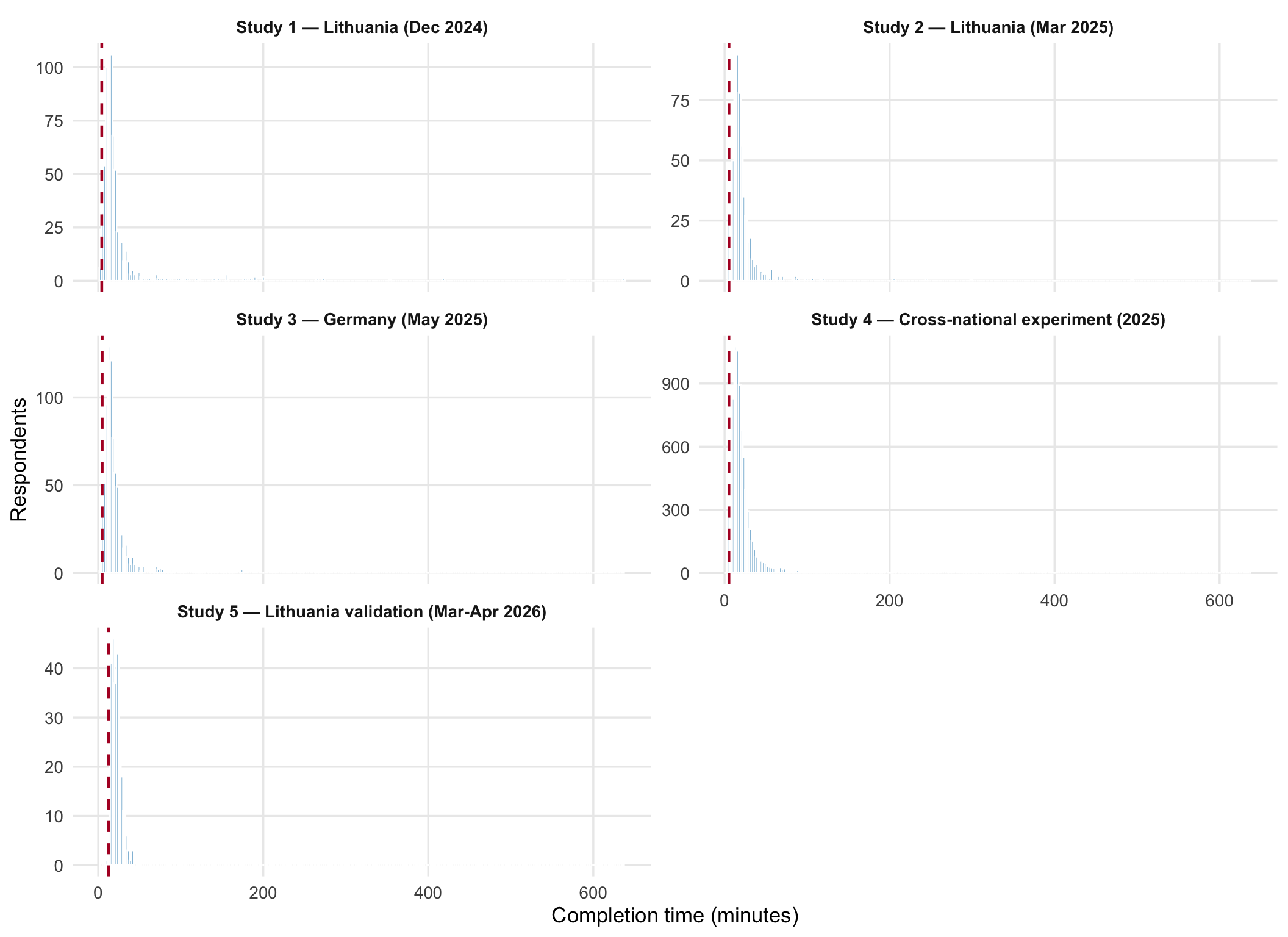
The cleaning script tags every respondent whose total duration falls below the 1st percentile via fast_completion. We report (a) the pooled distribution across studies and (b) per-study histograms so the reader can compare the shape of the panel samples (S1–S3) to the cross-national S4 wave and the SONA student pool in S5.

Code
duration_overview <- purrr::imap_dfr(items_data, ~ {
  tibble(
    study_code = .y,
    median_minutes = stats::median(.x$duration_minutes, na.rm = TRUE),
    p95_minutes = stats::quantile(.x$duration_minutes, probs = 0.95, na.rm = TRUE),
    fast_cases = sum(.x$fast_completion, na.rm = TRUE),
    fast_pct = mean(.x$fast_completion, na.rm = TRUE) * 100
  )
}) %>%
  dplyr::left_join(study_lookup, by = "study_code") %>%
  dplyr::mutate(label = dplyr::coalesce(label, study_code))

duration_overview %>%
  dplyr::mutate(
    median_minutes = round(median_minutes, 2),
    p95_minutes = round(p95_minutes, 2),
    fast_cases = scales::comma(fast_cases),
    fast_pct = scales::percent(fast_pct / 100, accuracy = 0.1)
  ) %>%
  dplyr::select(label, median_minutes, p95_minutes, fast_cases, fast_pct) %>%
  knitr::kable(
    col.names = c("Study", "Median minutes", "95th percentile", "Fast completions", "Fast share"),
    align = c("l", "r", "r", "r", "r")
  ) %>%
  kableExtra::kable_styling(full_width = FALSE)
Completion-time and speeding diagnostics by study
Study Median minutes 95th percentile Fast completions Fast share
Study 1 — Lithuania (Dec 2024) 15.57 97.50 6 0.9%
Study 2 — Lithuania (Mar 2025) 17.02 56.36 7 1.2%
Study 3 — Germany (May 2025) 15.88 75.87 5 0.6%
Study 4 — Cross-national experiment (2025) 17.07 59.65 72 0.9%
Study 5 — Lithuania validation (Mar-Apr 2026) 21.38 34.44 0 0.0%
Code
plot_duration_data <- purrr::imap_dfr(items_data, ~ {
  x_limit <- stats::quantile(.x$duration_minutes, probs = 0.99, na.rm = TRUE)
  tibble(
    study_code = .y,
    duration_minutes = .x$duration_minutes,
    fast_cut = stats::quantile(.x$duration_minutes, probs = 0.01, na.rm = TRUE),
    x_limit = x_limit
  )
}) %>%
  dplyr::left_join(study_lookup, by = "study_code") %>%
  dplyr::filter(is.finite(duration_minutes), duration_minutes >= 0, duration_minutes <= x_limit)

cutoffs <- plot_duration_data %>%
  dplyr::group_by(label) %>%
  dplyr::summarise(
    fast_cut = dplyr::first(fast_cut),
    x_limit = dplyr::first(x_limit),
    .groups = "drop"
  )

binwidth_global <- duration_histogram_binwidth(
  x = plot_duration_data$duration_minutes,
  x_limit = stats::quantile(plot_duration_data$duration_minutes, probs = 0.99, na.rm = TRUE)
)

ggplot(plot_duration_data, aes(x = duration_minutes)) +
  geom_histogram(binwidth = binwidth_global, fill = "#2B8CBE", color = "white", alpha = 0.85) +
  geom_vline(
    data = cutoffs,
    aes(xintercept = fast_cut),
    linetype = "dashed",
    linewidth = 0.8,
    color = "#B2182B"
  ) +
  facet_wrap(~ label, scales = "free_y", ncol = 2) +
  labs(x = "Completion time (minutes)", y = "Respondents") +
  theme(
    strip.text = element_text(face = "bold"),
    panel.grid.minor = element_blank()
  )

Pooled completion-time histograms by study. The dashed line marks each study’s 1st-percentile fast-completion cutoff.
  • Median completion times span 15.6 to 21.4 minutes — by design (S4/S5 carry larger batteries).
  • The maximum flagged speeding share is 1.2%, which is consistent with a low large-scale response-quality risk after cleaning. Per-study sensitivity checks against the fast_completion flag live in the modelling reports.

Item-level missingness

We surface the worst-case item-level missingness for each study so naming drift or unintentional item drop-outs cannot hide in the modelling stage. The cleaning script makes a CONSORT-style exclusion log; this table is the analogous item-level QA companion.

Study 1 — Lithuania (Dec 2024)
Study 1 — Lithuania (Dec 2024): 10 items with the highest missingness
Item Missing (%)
poi1 0
poi2 0
poi3 0
poi4 0
poi5 0
poi6 0
poi7 0
exp1 0
exp2 0
exp3 0
  • Median item missingness: 0%.
  • Worst-case item missingness: 0%. Study 2 — Lithuania (Mar 2025)
    Study 2 — Lithuania (Mar 2025): 10 items with the highest missingness
    Item Missing (%)
    gen1 0
    gen2 0
    gen3 0
    gen4 0
    gen5 0
    gen6 0
    gen7 0
    gen8 0
    th1 0
    th3 0
    • Median item missingness: 0%.
  • Worst-case item missingness: 0%. Study 3 — Germany (May 2025)
    Study 3 — Germany (May 2025): 10 items with the highest missingness
    Item Missing (%)
    gen1 0
    gen2 0
    gen3 0
    gen4 0
    gen5 0
    gen6 0
    gen7 0
    gen8 0
    th1 0
    th2 0
    • Median item missingness: 0%.
  • Worst-case item missingness: 0%. Study 4 — Cross-national experiment (2025)
    Study 4 — Cross-national experiment (2025): 10 items with the highest missingness
    Item Missing (%)
    q2_5 99.59
    q2_3 99.45
    q1_19_6 99.18
    q2_8 99.18
    q1_17_6 99.10
    q2_2 98.98
    q1_16_6 98.91
    q1_18_6 98.78
    q1_5_6 98.76
    q1_9_6 98.57
    • Median item missingness: 63.7%.
  • Worst-case item missingness: 99.59%. Study 5 — Lithuania validation (Mar-Apr 2026)
    Study 5 — Lithuania validation (Mar-Apr 2026): 10 items with the highest missingness
    Item Missing (%)
    pop6 0.4
    pop7 0.4
    pop8 0.4
    pop9 0.4
    pop10 0.4
    feel_ru 0.4
    feel_ch 0.4
    rwa4 0.4
    rwa5 0.4
    rwa6 0.4
    • Median item missingness: 0%.
  • Worst-case item missingness: 0.4%.

Item-level descriptives for the FIMI outcome

The FIMI news-evaluation items are the dependent variable of every Study 1–4 model, so their item-level distribution matters more than for any other scale. We list mean / SD / median / min / max / missingness for every news* indicator that survived the cleaning stage.

Item-level descriptives for the FIMI news-evaluation battery (S1–S4)
Study Item n Mean SD Median Min Max Missing (%)
Study 1 — Lithuania (Dec 2024) news1 681 3.03 2.05 3.0 1 7 0
Study 1 — Lithuania (Dec 2024) news2 681 3.54 2.20 4.0 1 7 0
Study 1 — Lithuania (Dec 2024) news3 681 2.84 2.21 2.0 1 7 0
Study 1 — Lithuania (Dec 2024) news4 681 2.75 2.02 2.0 1 7 0
Study 1 — Lithuania (Dec 2024) news5 681 2.66 1.88 2.0 1 7 0
Study 1 — Lithuania (Dec 2024) news6 681 2.28 1.79 1.0 1 7 0
Study 1 — Lithuania (Dec 2024) news7 681 2.39 1.89 1.0 1 7 0
Study 1 — Lithuania (Dec 2024) news8 681 2.67 1.92 2.0 1 7 0
Study 1 — Lithuania (Dec 2024) news9 681 2.45 1.97 1.0 1 7 0
Study 1 — Lithuania (Dec 2024) news10 681 2.49 1.96 1.0 1 7 0
Study 1 — Lithuania (Dec 2024) news11 681 3.01 2.25 2.0 1 7 0
Study 1 — Lithuania (Dec 2024) news12 681 2.75 1.98 2.0 1 7 0
Study 1 — Lithuania (Dec 2024) news13 681 3.01 2.18 2.0 1 7 0
Study 1 — Lithuania (Dec 2024) news14 681 2.61 1.80 2.0 1 7 0
Study 1 — Lithuania (Dec 2024) news15 681 2.33 1.72 1.0 1 7 0
Study 2 — Lithuania (Mar 2025) news1 582 6.01 1.67 7.0 1 7 0
Study 2 — Lithuania (Mar 2025) news2 582 5.61 1.74 6.5 1 7 0
Study 2 — Lithuania (Mar 2025) news3 582 5.26 1.85 6.0 1 7 0
Study 2 — Lithuania (Mar 2025) news4 582 4.96 1.82 5.0 1 7 0
Study 2 — Lithuania (Mar 2025) news5 582 5.71 1.73 7.0 1 7 0
Study 2 — Lithuania (Mar 2025) news6 582 4.75 1.95 4.5 1 7 0
Study 2 — Lithuania (Mar 2025) news7 582 4.54 1.70 4.0 1 7 0
Study 2 — Lithuania (Mar 2025) news8 582 4.96 1.64 4.0 1 7 0
Study 3 — Germany (May 2025) news1 782 5.34 1.88 6.0 1 7 0
Study 3 — Germany (May 2025) news2 782 5.13 1.89 5.5 1 7 0
Study 3 — Germany (May 2025) news3 782 3.31 1.88 3.0 1 7 0
Study 3 — Germany (May 2025) news4 782 4.58 1.68 4.0 1 7 0
Study 3 — Germany (May 2025) news5 782 5.48 1.74 6.0 1 7 0
Study 3 — Germany (May 2025) news6 782 4.53 1.94 4.0 1 7 0
Study 3 — Germany (May 2025) news7 782 4.23 1.70 4.0 1 7 0
Study 3 — Germany (May 2025) news8 782 4.49 1.88 4.0 1 7 0
Study 4 — Cross-national experiment (2025) news1 8040 5.56 1.76 6.0 1 7 0
Study 4 — Cross-national experiment (2025) news2 8040 5.07 1.81 5.0 1 7 0
Study 4 — Cross-national experiment (2025) news3 8040 4.58 1.87 5.0 1 7 0
Study 4 — Cross-national experiment (2025) news4 8040 4.79 1.71 5.0 1 7 0
Study 4 — Cross-national experiment (2025) news5 8040 5.41 1.74 6.0 1 7 0
Study 4 — Cross-national experiment (2025) news6 8040 4.47 1.83 4.0 1 7 0
Study 4 — Cross-national experiment (2025) news7 8040 4.28 1.67 4.0 1 7 0
Study 4 — Cross-national experiment (2025) news8 8040 4.68 1.70 5.0 1 7 0

Scale-level reliability and descriptives

The pooled reliability + descriptives table below is the single source of truth for every alpha / omega / AVE figure quoted later in the manuscript. We split the role column up-front so the outcome (FIMI) rows can be picked out at a glance from the DisInformeter scale predictors and the validation / COND rows.

Code
scale_summary_all %>%
  dplyr::mutate(
    scale = stringr::str_to_upper(scale),
    across(c(alpha, omega, avg_r, ave, mean, sd, median, mad, min, max), ~ round(.x, 2)),
    missing_pct = scales::percent(missing_pct / 100, accuracy = 0.01)
  ) %>%
  dplyr::arrange(label, dplyr::desc(role == "outcome (DV — FIMI)"), role, scale) %>%
  dplyr::select(label, role, scale, n_items, n_observations,
                alpha, omega, avg_r, ave, mean, sd, median, mad, min, max, missing_pct) %>%
  knitr::kable(
    col.names = c("Study", "Role", "Scale", "Items", "n",
                  "Cronbach's α", "Omega", "Avg. r", "AVE",
                  "Mean", "SD", "Median", "MAD", "Min", "Max", "Missing"),
    align = c("l", "l", "l", rep("r", 13))
  ) %>%
  kableExtra::kable_styling(full_width = FALSE, font_size = 9) %>%
  kableExtra::scroll_box(height = "560px")
Reliability and score descriptives by study and scale
Study Role Scale Items n Cronbach's α Omega Avg. r AVE Mean SD Median MAD Min Max Missing
Study 1 — Lithuania (Dec 2024) outcome (DV — FIMI) FIMI 15 681 0.93 0.93 0.47 0.48 2.72 1.42 2.53 1.20 1.00 7.00 0.00%
Study 1 — Lithuania (Dec 2024) outcome (DV — FIMI) FIMI_SHORT 4 681 0.81 0.82 0.53 0.54 2.54 1.51 2.25 1.25 1.00 7.00 0.00%
Study 1 — Lithuania (Dec 2024) DisInformeter scale predictor ANXK 5 681 0.92 0.92 0.70 0.70 3.74 1.84 3.80 1.40 1.00 7.00 0.00%
Study 1 — Lithuania (Dec 2024) DisInformeter scale predictor ANXR 5 681 0.92 0.93 0.71 0.71 3.09 1.97 2.60 1.60 1.00 7.00 0.00%
Study 1 — Lithuania (Dec 2024) DisInformeter scale predictor FEAR 2 681 0.79 0.79 0.66 0.66 4.03 2.05 4.00 1.50 1.00 7.00 0.00%
Study 1 — Lithuania (Dec 2024) DisInformeter scale predictor GAY 3 681 0.90 0.91 0.76 0.78 4.70 2.07 5.00 2.00 1.00 7.00 0.00%
Study 1 — Lithuania (Dec 2024) DisInformeter scale predictor LEFT 2 681 0.79 0.80 0.66 0.66 3.69 1.87 3.50 1.50 1.00 7.00 0.00%
Study 1 — Lithuania (Dec 2024) DisInformeter scale predictor LONE 4 681 0.92 0.92 0.73 0.73 3.79 1.88 3.75 1.50 1.00 7.00 0.00%
Study 1 — Lithuania (Dec 2024) DisInformeter scale predictor MIGR 2 681 0.82 0.82 0.70 0.70 4.85 1.71 5.00 1.50 1.00 7.00 0.00%
Study 1 — Lithuania (Dec 2024) DisInformeter scale predictor RULE 2 681 0.78 0.78 0.65 0.65 3.04 1.82 2.50 1.50 1.00 7.00 0.00%
Study 1 — Lithuania (Dec 2024) DisInformeter scale predictor SAFE 3 681 0.83 0.83 0.63 0.63 3.30 1.80 3.00 1.33 1.00 7.00 0.00%
Study 1 — Lithuania (Dec 2024) DisInformeter scale predictor SUPK 10 681 0.95 0.95 0.63 0.63 3.72 1.54 3.90 1.10 1.00 7.00 0.00%
Study 1 — Lithuania (Dec 2024) DisInformeter scale predictor SUPR 12 681 0.96 0.96 0.69 0.66 2.74 1.70 2.25 1.17 1.00 7.00 0.00%
Study 1 — Lithuania (Dec 2024) DisInformeter scale predictor THREAT 2 681 0.80 0.80 0.67 0.67 3.91 2.08 4.00 2.00 1.00 7.00 0.00%
Study 1 — Lithuania (Dec 2024) DisInformeter scale predictor USE 6 681 0.92 0.92 0.66 0.66 3.79 1.77 3.67 1.33 1.00 7.00 0.00%
Study 2 — Lithuania (Mar 2025) outcome (DV — FIMI) FIMI 8 582 0.78 0.79 0.31 0.32 5.22 1.11 5.25 0.75 1.00 7.00 0.00%
Study 2 — Lithuania (Mar 2025) outcome (DV — FIMI) FIMI_SHORT 4 582 0.69 0.69 0.36 0.36 5.20 1.22 5.25 1.00 1.00 7.00 0.00%
Study 2 — Lithuania (Mar 2025) DisInformeter scale predictor ABAND 3 582 0.80 0.80 0.57 0.56 3.80 1.67 4.00 1.33 1.00 7.00 0.00%
Study 2 — Lithuania (Mar 2025) DisInformeter scale predictor ABANF 4 582 0.91 0.91 0.71 0.71 3.84 1.67 4.00 1.25 1.00 7.00 0.00%
Study 2 — Lithuania (Mar 2025) DisInformeter scale predictor ABANH 5 582 0.93 0.93 0.71 0.72 3.89 1.84 4.00 1.60 1.00 7.00 0.00%
Study 2 — Lithuania (Mar 2025) DisInformeter scale predictor ABANM 4 582 0.95 0.95 0.82 0.83 3.57 1.94 3.75 1.62 1.00 7.00 0.00%
Study 2 — Lithuania (Mar 2025) DisInformeter scale predictor EXPL 4 582 0.90 0.90 0.70 0.70 3.85 1.70 4.00 1.25 1.00 7.00 0.00%
Study 2 — Lithuania (Mar 2025) DisInformeter scale predictor GAY 3 582 0.94 0.94 0.84 0.84 4.35 2.14 4.33 2.00 1.00 7.00 0.00%
Study 2 — Lithuania (Mar 2025) DisInformeter scale predictor MIGR 3 582 0.90 0.90 0.75 0.76 5.11 1.61 5.33 1.33 1.00 7.00 0.00%
Study 2 — Lithuania (Mar 2025) DisInformeter scale predictor PRAG 2 582 0.75 0.75 0.60 0.60 4.33 1.92 4.50 1.50 1.00 7.00 0.00%
Study 2 — Lithuania (Mar 2025) DisInformeter scale predictor PRAGR 4 582 0.90 0.90 0.69 0.69 3.02 1.86 2.62 1.62 1.00 7.00 0.00%
Study 2 — Lithuania (Mar 2025) DisInformeter scale predictor SUPF 3 582 0.94 0.94 0.84 0.84 1.92 1.53 1.00 0.00 1.00 7.00 0.00%
Study 2 — Lithuania (Mar 2025) DisInformeter scale predictor SUPR 6 582 0.93 0.93 0.70 0.70 2.34 1.56 1.75 0.75 1.00 7.00 0.00%
Study 2 — Lithuania (Mar 2025) DisInformeter scale predictor THREAT 3 582 0.73 0.74 0.48 0.47 4.05 1.63 4.00 1.00 1.00 7.00 0.00%
Study 3 — Germany (May 2025) outcome (DV — FIMI) FIMI 8 782 0.55 0.56 0.13 0.14 4.64 0.89 4.62 0.62 1.00 7.00 0.00%
Study 3 — Germany (May 2025) outcome (DV — FIMI) FIMI_SHORT 4 782 0.40 0.41 0.14 0.16 4.83 1.08 4.75 0.75 1.00 7.00 0.00%
Study 3 — Germany (May 2025) DisInformeter scale predictor ABAND 3 782 0.82 0.82 0.61 0.60 3.72 1.73 3.67 1.33 1.00 7.00 0.00%
Study 3 — Germany (May 2025) DisInformeter scale predictor ABANF 4 782 0.91 0.91 0.71 0.72 3.29 1.63 3.25 1.25 1.00 7.00 0.00%
Study 3 — Germany (May 2025) DisInformeter scale predictor ABANH 5 782 0.94 0.94 0.76 0.77 3.82 1.92 3.80 1.60 1.00 7.00 0.00%
Study 3 — Germany (May 2025) DisInformeter scale predictor ABANM 4 782 0.95 0.95 0.83 0.83 3.20 1.96 3.00 1.75 1.00 7.00 0.00%
Study 3 — Germany (May 2025) DisInformeter scale predictor EXPL 4 782 0.87 0.88 0.63 0.63 3.66 1.62 3.75 1.25 1.00 7.00 0.00%
Study 3 — Germany (May 2025) DisInformeter scale predictor GAY 3 782 0.96 0.96 0.88 0.88 2.85 1.96 2.33 1.33 1.00 7.00 0.00%
Study 3 — Germany (May 2025) DisInformeter scale predictor MIGR 3 782 0.95 0.95 0.85 0.85 4.25 2.02 4.33 1.67 1.00 7.00 0.00%
Study 3 — Germany (May 2025) DisInformeter scale predictor PRAG 2 782 0.84 0.84 0.72 0.72 4.04 2.02 4.00 1.50 1.00 7.00 0.00%
Study 3 — Germany (May 2025) DisInformeter scale predictor PRAGR 4 782 0.91 0.91 0.72 0.72 3.48 1.91 3.50 1.75 1.00 7.00 0.00%
Study 3 — Germany (May 2025) DisInformeter scale predictor SUPF 3 782 0.88 0.90 0.73 0.76 2.36 1.63 1.67 0.67 1.00 7.00 0.00%
Study 3 — Germany (May 2025) DisInformeter scale predictor SUPR 6 782 0.92 0.92 0.65 0.63 2.93 1.58 2.67 1.33 1.00 7.00 0.00%
Study 3 — Germany (May 2025) DisInformeter scale predictor THREAT 3 782 0.75 0.76 0.51 0.52 3.35 1.67 3.33 1.33 1.00 7.00 0.00%
Study 4 — Cross-national experiment (2025) outcome (DV — FIMI) FIMI 8 8040 0.69 0.69 0.22 0.23 4.86 0.99 4.88 0.62 1.00 7.00 0.00%
Study 4 — Cross-national experiment (2025) outcome (DV — FIMI) FIMI_SHORT 4 8040 0.53 0.53 0.22 0.23 4.86 1.11 4.75 0.75 1.00 7.00 0.00%
Study 4 — Cross-national experiment (2025) COND experimental outcome CLICK_REASONS 6 8040 0.86 0.86 0.50 0.51 3.99 1.39 4.00 0.83 1.00 7.00 0.00%
Study 4 — Cross-national experiment (2025) COND experimental outcome DEM_IMPORT 1 8040 NA NA NA NA 9.25 2.24 10.00 1.00 1.00 11.00 0.00%
Study 4 — Cross-national experiment (2025) COND experimental outcome EU_SUPPORT 1 8040 NA NA NA NA 6.84 3.28 7.00 2.00 1.00 12.00 0.00%
Study 4 — Cross-national experiment (2025) COND experimental outcome INST_TRUST 8 8040 0.90 0.90 0.53 0.53 5.51 2.19 5.62 1.50 1.00 11.00 0.00%
Study 4 — Cross-national experiment (2025) COND experimental outcome LIFE_SAT 1 8040 NA NA NA NA 6.66 2.48 7.00 2.00 1.00 11.00 0.00%
Study 4 — Cross-national experiment (2025) COND experimental outcome LR_SCALE 1 8040 NA NA NA NA 6.33 2.36 6.00 1.00 1.00 11.00 0.00%
Study 4 — Cross-national experiment (2025) COND experimental outcome MEDIA_FREQ 5 8040 0.61 0.62 0.23 0.26 4.16 1.26 4.20 0.80 1.00 7.00 0.00%
Study 4 — Cross-national experiment (2025) COND experimental outcome MISINFO_ACTION 6 8040 NA NA NA NA 1.72 0.95 1.00 0.00 0.00 6.00 0.00%
Study 4 — Cross-national experiment (2025) COND experimental outcome MISINFO_CONF 1 8040 NA NA NA NA 5.01 1.49 5.00 1.00 1.00 7.00 0.00%
Study 4 — Cross-national experiment (2025) COND experimental outcome MISINFO_FOREIGN 9 8040 0.89 0.89 0.47 0.47 4.45 1.11 4.44 0.67 1.00 7.00 0.00%
Study 4 — Cross-national experiment (2025) COND experimental outcome MISINFO_FREE 1 8040 NA NA NA NA 4.36 1.76 4.00 1.00 1.00 7.00 0.00%
Study 4 — Cross-national experiment (2025) COND experimental outcome MISINFO_IMPACT 6 8040 0.90 0.90 0.59 0.60 4.72 1.32 4.67 0.83 1.00 7.00 0.00%
Study 4 — Cross-national experiment (2025) COND experimental outcome MISINFO_POL 1 8040 NA NA NA NA 5.20 1.43 5.00 1.00 1.00 7.00 0.00%
Study 4 — Cross-national experiment (2025) COND experimental outcome MISINFO_REGUL 2 8040 0.65 0.65 0.48 0.48 5.25 1.27 5.50 0.50 1.00 7.00 0.00%
Study 4 — Cross-national experiment (2025) COND experimental outcome MISINFO_RESP 9 8040 0.94 0.94 0.63 0.64 5.40 1.29 5.56 1.00 1.00 7.00 0.00%
Study 4 — Cross-national experiment (2025) COND experimental outcome MISINFO_SRC 9 8040 0.89 0.89 0.48 0.49 4.74 1.10 4.78 0.78 1.00 7.00 0.00%
Study 4 — Cross-national experiment (2025) COND experimental outcome POL_EFF_EXT 1 8040 NA NA NA NA 2.05 0.91 2.00 1.00 1.00 4.00 0.00%
Study 4 — Cross-national experiment (2025) COND experimental outcome POL_EFF_INT 1 8040 NA NA NA NA 2.34 1.13 2.00 1.00 1.00 5.00 0.00%
Study 4 — Cross-national experiment (2025) COND experimental outcome POL_INTEREST 1 8040 NA NA NA NA 2.34 0.87 2.00 1.00 1.00 4.00 0.00%
Study 4 — Cross-national experiment (2025) COND experimental outcome POL_PARTIC 8 8040 NA NA NA NA 1.09 1.33 1.00 1.00 0.00 8.00 0.00%
Study 4 — Cross-national experiment (2025) COND experimental outcome RELIGIOSITY 1 8040 NA NA NA NA 5.23 3.12 6.00 3.00 1.00 11.00 0.00%
Study 4 — Cross-national experiment (2025) COND experimental outcome SOC_TRUST 3 8040 0.80 0.81 0.58 0.58 6.44 2.30 6.67 1.67 2.00 12.33 0.00%
Study 4 — Cross-national experiment (2025) DisInformeter scale predictor ABAND 3 8040 0.76 0.76 0.51 0.51 4.43 1.55 4.33 1.00 1.00 7.00 0.00%
Study 4 — Cross-national experiment (2025) DisInformeter scale predictor ABAND_LONG 6 8040 0.87 0.87 0.52 0.53 4.37 1.46 4.33 1.00 1.00 7.00 0.00%
Study 4 — Cross-national experiment (2025) DisInformeter scale predictor GEN 5 8040 0.63 0.65 0.25 0.31 4.05 1.16 4.00 0.80 1.00 7.00 0.00%
Study 4 — Cross-national experiment (2025) DisInformeter scale predictor PRAG 1 8040 NA NA NA NA 4.68 1.91 5.00 1.00 1.00 7.00 0.00%
Study 4 — Cross-national experiment (2025) DisInformeter scale predictor PRAG_LONG 3 8040 0.71 0.76 0.46 0.54 4.95 1.42 5.00 1.00 1.00 7.00 0.00%
Study 4 — Cross-national experiment (2025) DisInformeter scale predictor SUPCH 3 8040 0.94 0.94 0.83 0.83 3.04 1.78 3.00 1.67 1.00 7.00 0.00%
Study 4 — Cross-national experiment (2025) DisInformeter scale predictor SUPR 3 8040 0.95 0.95 0.86 0.86 2.70 1.87 2.00 1.00 1.00 7.00 0.00%
Study 4 — Cross-national experiment (2025) DisInformeter scale predictor THREAT 2 8040 0.53 0.54 0.37 0.39 4.40 1.65 4.50 1.00 1.00 7.00 0.00%
Study 4 — Cross-national experiment (2025) DisInformeter scale predictor THREAT_LONG 7 8040 0.86 0.86 0.46 0.47 4.64 1.41 4.71 1.00 1.00 7.00 0.00%
Study 5 — Lithuania validation (Mar-Apr 2026) DisInformeter scale predictor ABAND 8 248 0.87 0.87 0.45 0.36 3.11 1.19 3.00 0.75 1.00 6.62 0.00%
Study 5 — Lithuania validation (Mar-Apr 2026) DisInformeter scale predictor ABAN_STATE 5 248 0.92 0.92 0.71 0.71 2.66 1.43 2.20 0.80 1.00 7.00 0.00%
Study 5 — Lithuania validation (Mar-Apr 2026) DisInformeter scale predictor CEN 6 248 0.94 0.94 0.72 0.72 2.41 1.50 1.83 0.83 1.00 7.00 0.00%
Study 5 — Lithuania validation (Mar-Apr 2026) DisInformeter scale predictor CET 8 248 0.79 0.79 0.31 0.44 3.57 0.98 3.62 0.75 1.00 6.25 0.00%
Study 5 — Lithuania validation (Mar-Apr 2026) DisInformeter scale predictor EXPL 5 248 0.78 0.78 0.41 0.44 3.02 1.15 3.00 0.80 1.00 6.60 0.00%
Study 5 — Lithuania validation (Mar-Apr 2026) DisInformeter scale predictor FEAR 6 248 0.83 0.84 0.46 0.53 4.50 1.34 4.50 0.83 1.00 7.00 0.00%
Study 5 — Lithuania validation (Mar-Apr 2026) DisInformeter scale predictor GAY 6 248 0.91 0.92 0.66 0.82 2.73 1.61 2.17 1.00 1.00 7.00 0.00%
Study 5 — Lithuania validation (Mar-Apr 2026) DisInformeter scale predictor GEN 8 248 0.57 0.66 0.16 0.28 3.16 0.78 3.12 0.50 1.00 6.50 0.00%
Study 5 — Lithuania validation (Mar-Apr 2026) DisInformeter scale predictor MIGR 7 248 0.90 0.90 0.55 0.77 3.05 1.30 2.86 0.86 1.00 6.57 0.00%
Study 5 — Lithuania validation (Mar-Apr 2026) DisInformeter scale predictor PRAGCH 6 248 0.87 0.87 0.53 0.53 3.02 1.46 2.92 1.08 1.00 7.00 0.00%
Study 5 — Lithuania validation (Mar-Apr 2026) DisInformeter scale predictor PRAGR 6 248 0.86 0.87 0.52 0.58 2.24 1.32 2.00 0.83 1.00 7.00 0.00%
Study 5 — Lithuania validation (Mar-Apr 2026) DisInformeter scale predictor SUPCH 11 248 0.91 0.91 0.48 0.55 3.18 1.22 3.09 0.82 1.00 7.00 0.00%
Study 5 — Lithuania validation (Mar-Apr 2026) DisInformeter scale predictor SUPR 12 248 0.92 0.93 0.51 0.55 1.77 0.97 1.50 0.50 1.00 6.17 0.00%
Study 5 — Lithuania validation (Mar-Apr 2026) DisInformeter scale predictor SUP_GEN 8 248 0.92 0.93 0.64 0.64 1.78 1.14 1.25 0.25 1.00 7.00 0.00%
Study 5 — Lithuania validation (Mar-Apr 2026) DisInformeter scale predictor THREAT 12 248 0.85 0.85 0.31 0.32 3.49 1.15 3.42 0.92 1.17 6.83 0.00%
Study 5 — Lithuania validation (Mar-Apr 2026) DisInformeter scale predictor THREAT_FT 3 248 0.71 0.75 0.44 0.53 3.44 1.44 3.33 1.00 1.00 7.00 0.00%
Study 5 — Lithuania validation (Mar-Apr 2026) DisInformeter scale predictor THREAT_GAY 3 248 0.97 0.97 0.91 0.91 2.51 1.88 1.67 0.67 1.00 7.00 0.00%
Study 5 — Lithuania validation (Mar-Apr 2026) DisInformeter scale predictor THREAT_MIGR 2 248 0.90 0.90 0.82 0.82 3.70 1.85 3.50 1.50 1.00 7.00 0.00%
Study 5 — Lithuania validation (Mar-Apr 2026) DisInformeter scale predictor UNP 4 248 0.87 0.87 0.62 0.64 2.85 1.32 2.50 1.00 1.00 7.00 0.00%
Study 5 — Lithuania validation (Mar-Apr 2026) validation battery CMQ 5 248 0.84 0.84 0.51 0.52 6.69 2.22 6.80 1.60 1.00 11.00 0.00%
Study 5 — Lithuania validation (Mar-Apr 2026) validation battery FEEL_CH 1 247 NA NA NA NA 21.08 22.77 15.00 15.00 0.00 100.00 0.40%
Study 5 — Lithuania validation (Mar-Apr 2026) validation battery FEEL_EU 1 248 NA NA NA NA 81.37 17.64 85.00 10.00 0.00 100.00 0.00%
Study 5 — Lithuania validation (Mar-Apr 2026) validation battery FEEL_NATO 1 248 NA NA NA NA 73.88 22.66 80.00 12.00 0.00 100.00 0.00%
Study 5 — Lithuania validation (Mar-Apr 2026) validation battery FEEL_RU 1 247 NA NA NA NA 5.22 15.09 0.00 0.00 0.00 100.00 0.40%
Study 5 — Lithuania validation (Mar-Apr 2026) validation battery ITT_IMI 6 248 0.94 0.94 0.72 0.72 2.81 1.51 2.50 1.17 1.00 7.00 0.00%
Study 5 — Lithuania validation (Mar-Apr 2026) validation battery ITT_IMI_REAL 3 248 0.93 0.93 0.81 0.81 2.97 1.64 2.67 1.33 1.00 7.00 0.00%
Study 5 — Lithuania validation (Mar-Apr 2026) validation battery ITT_IMI_SYM 3 248 0.96 0.97 0.90 0.90 2.66 1.65 2.00 1.00 1.00 7.00 0.00%
Study 5 — Lithuania validation (Mar-Apr 2026) validation battery ITT_LGBT 8 248 0.93 0.93 0.62 0.63 2.23 1.39 1.75 0.75 1.00 7.00 0.00%
Study 5 — Lithuania validation (Mar-Apr 2026) validation battery ITT_LGBT_REAL 4 248 0.82 0.84 0.56 0.57 1.90 1.24 1.25 0.25 1.00 7.00 0.00%
Study 5 — Lithuania validation (Mar-Apr 2026) validation battery ITT_LGBT_SYM 4 248 0.94 0.95 0.82 0.82 2.56 1.73 2.00 1.00 1.00 7.00 0.00%
Study 5 — Lithuania validation (Mar-Apr 2026) validation battery PANAS_NA 5 247 0.81 0.82 0.46 0.48 3.42 1.08 3.40 0.80 1.20 6.60 0.40%
Study 5 — Lithuania validation (Mar-Apr 2026) validation battery PANAS_PA 5 248 0.73 0.74 0.36 0.38 4.84 0.93 5.00 0.60 1.80 7.00 0.00%
Study 5 — Lithuania validation (Mar-Apr 2026) validation battery POP 9 248 0.40 0.46 0.08 0.12 4.66 0.62 4.67 0.44 3.00 6.22 0.00%
Study 5 — Lithuania validation (Mar-Apr 2026) validation battery POP_ELITE 3 248 0.27 0.48 0.11 0.37 4.53 0.95 4.67 0.67 1.67 7.00 0.00%
Study 5 — Lithuania validation (Mar-Apr 2026) validation battery POP_MANI 3 247 0.18 0.45 0.07 0.36 3.84 1.03 4.00 0.67 1.00 6.67 0.40%
Study 5 — Lithuania validation (Mar-Apr 2026) validation battery POP_PEOPLE 3 248 0.36 0.49 0.19 0.30 5.60 0.90 5.67 0.67 2.67 7.00 0.00%
Study 5 — Lithuania validation (Mar-Apr 2026) validation battery RWA 6 248 0.56 0.63 0.15 0.27 3.95 1.28 3.83 1.00 1.00 7.67 0.00%
Study 5 — Lithuania validation (Mar-Apr 2026) validation battery TRUST_EU 1 248 NA NA NA NA 6.16 2.10 7.00 1.00 1.00 10.00 0.00%
Study 5 — Lithuania validation (Mar-Apr 2026) validation battery TRUST_LOCAL 5 248 0.86 0.86 0.55 0.55 4.98 1.63 5.00 1.20 1.00 9.20 0.00%
Study 5 — Lithuania validation (Mar-Apr 2026) validation battery TRUST_UN 1 248 NA NA NA NA 5.67 2.62 6.00 2.00 1.00 10.00 0.00%
  • Across all study-scale combinations, the median alpha is 0.87 and median omega is 0.87.
  • The highest scale-level missingness is 0.40%.
  • As expected, single-item or two-item scales (especially in the S4 outcome battery and S5 validation thermometers) show attenuated alpha, so omega and AVE are reported in parallel for transparency.

Scale-score distributions

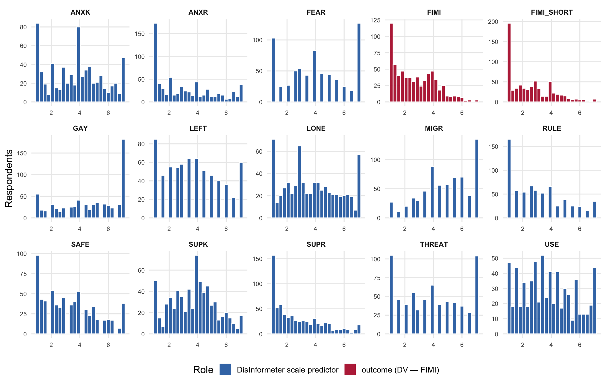
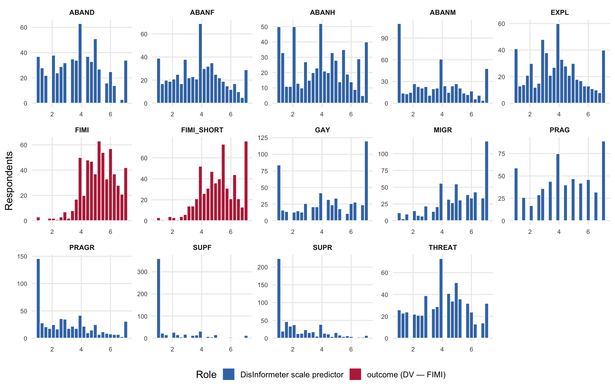
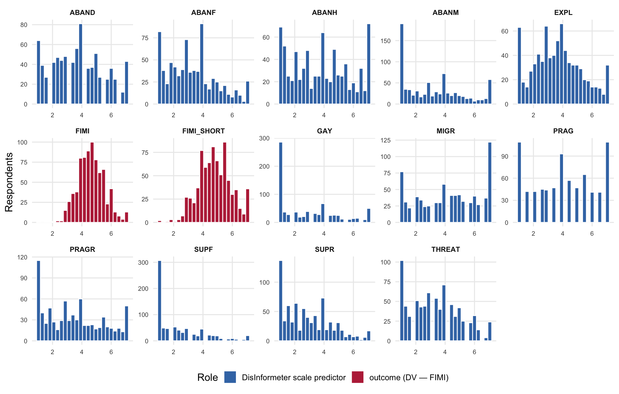
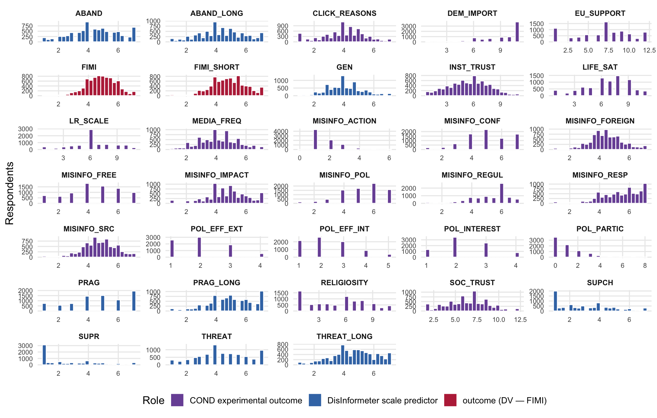
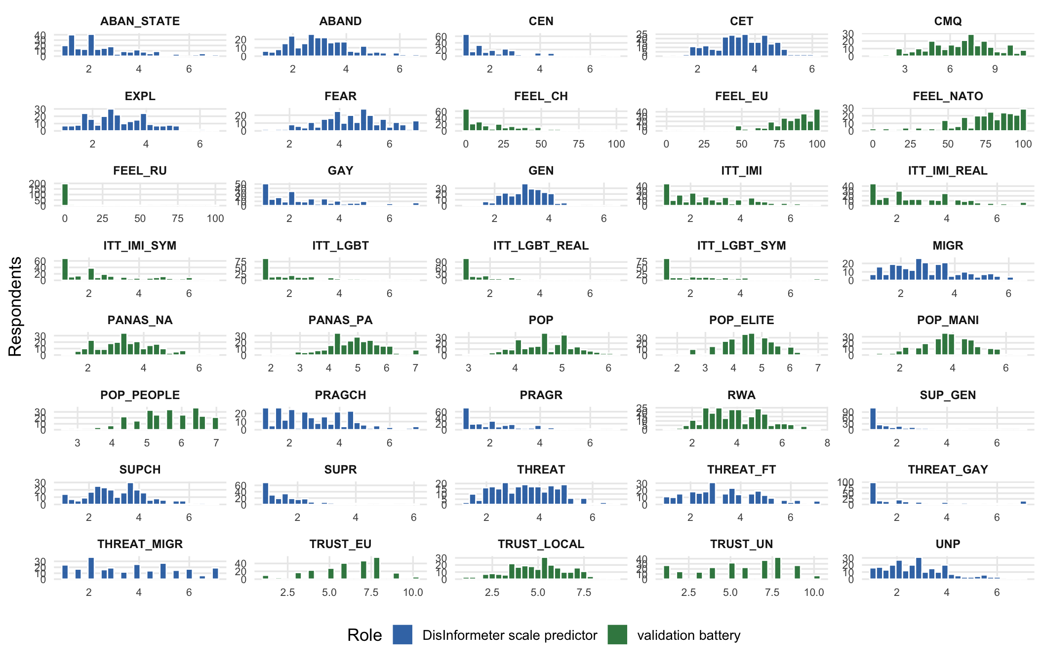
Beyond a single point estimate per scale, we visualise the full empirical distribution of every scored construct in every study. Histograms are faceted by scale (one mini panel per construct) so attenuated, skewed, or floor / ceiling distributions stay visible to the reader.

Study 1 — Lithuania (Dec 2024): scale score histograms

Study 2 — Lithuania (Mar 2025): scale score histograms

Study 3 — Germany (May 2025): scale score histograms

Study 4 — Cross-national experiment (2025): scale score histograms

Study 5 — Lithuania validation (Mar-Apr 2026): scale score histograms

Cross-study comparable constructs

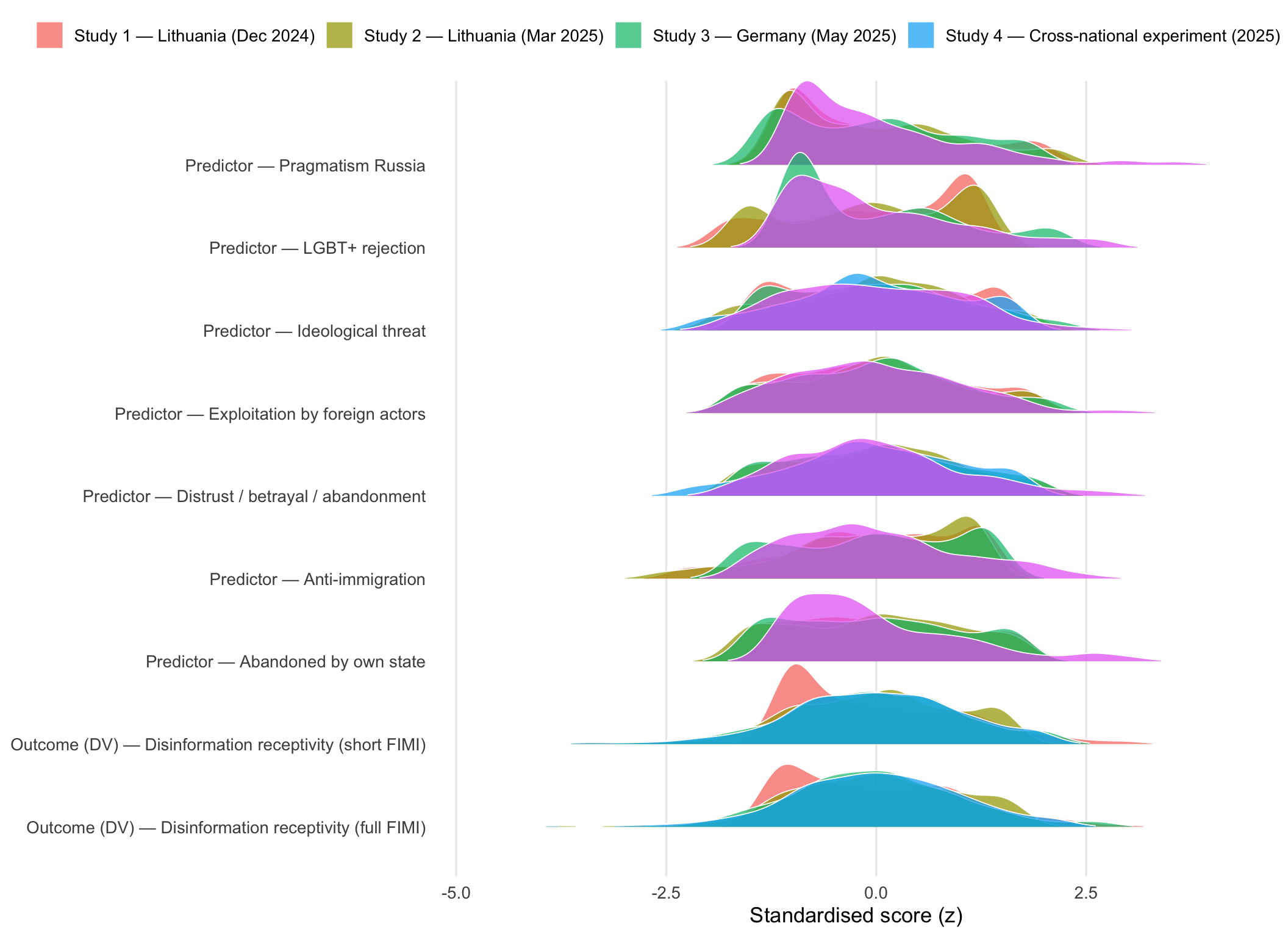
Several DisInformeter sub-scales recur across waves with broadly comparable item sets. We standardise scores within each study × scale (z-score) before stacking, so the resulting ridge plot shows distributional shape and dispersion on a common axis without being dragged around by metric drift between Likert anchors. Constructs whose item sets diverge too much across waves (S1’s two-item proto-FEAR vs S5’s six-item FEAR; S1’s two-item RULE vs S2/S3’s three-item admiration SUPF; …) are deliberately omitted here so the figure does not over-suggest invariance — those scales live in the per-study tables above. The crosswalk below documents the legacy S1 labels (USE, LONE, ANXR, …) and the legacy S5 wrangled-scale name (ABAN_STATE) explicitly — these are the per-wave Layer-2 scale-score column names, retained here for historical traceability; the canonical latent labels carried by R/sem_specs.R are EXPL, ABANH, PRAGR, …

Code
construct_map <- tibble::tribble(
  ~role, ~construct, ~S1, ~S2, ~S3, ~S4, ~S5,
  "Outcome (DV)",   "Disinformation receptivity (full FIMI)",  "FIMI",       "FIMI",       "FIMI",       "FIMI",       NA,
  "Outcome (DV)",   "Disinformation receptivity (short FIMI)", "FIMI_SHORT", "FIMI_SHORT", "FIMI_SHORT", "FIMI_SHORT", NA,
  "Predictor",      "Ideological threat",                          "THREAT",     "THREAT",     "THREAT",     "THREAT",     "THREAT",
  "Predictor",      "Exploitation by foreign actors",              "USE",        "EXPL",       "EXPL",       NA,           "EXPL",
  "Predictor",      "Anti-immigration",                            "MIGR",       "MIGR",       "MIGR",       NA,           "MIGR",
  "Predictor",      "LGBT+ rejection",                             "GAY",        "GAY",        "GAY",        NA,           "GAY",
  "Predictor",      "Pragmatism Russia",                           "ANXR",       "PRAGR",      "PRAGR",      NA,           "PRAGR",
  "Predictor",      "Distrust / betrayal / abandonment",           NA,           "ABAND",      "ABAND",      "ABAND",      "ABAND",
  "Predictor",      "Abandoned by own state",                      "LONE",       "ABANH",      "ABANH",      NA,           "ABAN_STATE"
)

construct_map %>%
  knitr::kable(align = c("l", "l", "c", "c", "c", "c", "c")) %>%
  kableExtra::kable_styling(full_width = FALSE)
Cross-study mapping for key comparable constructs
role construct S1 S2 S3 S4 S5
Outcome (DV) Disinformation receptivity (full FIMI) FIMI FIMI FIMI FIMI NA
Outcome (DV) Disinformation receptivity (short FIMI) FIMI_SHORT FIMI_SHORT FIMI_SHORT FIMI_SHORT NA
Predictor Ideological threat THREAT THREAT THREAT THREAT THREAT
Predictor Exploitation by foreign actors USE EXPL EXPL NA EXPL
Predictor Anti-immigration MIGR MIGR MIGR NA MIGR
Predictor LGBT+ rejection GAY GAY GAY NA GAY
Predictor Pragmatism Russia ANXR PRAGR PRAGR NA PRAGR
Predictor Distrust / betrayal / abandonment NA ABAND ABAND ABAND ABAND
Predictor Abandoned by own state LONE ABANH ABANH NA ABAN_STATE
Code
scale_long <- purrr::imap_dfr(scales_data, ~ {
  .x %>%
    dplyr::select(dplyr::starts_with("scale_")) %>%
    tidyr::pivot_longer(
      cols = dplyr::everything(),
      names_to = "scale",
      values_to = "value",
      names_prefix = "scale_"
    ) %>%
    dplyr::mutate(study_code = .y, scale = stringr::str_to_upper(scale))
})

construct_long <- construct_map %>%
  tidyr::pivot_longer(
    cols = c(S1, S2, S3, S4, S5),
    names_to = "study_code",
    values_to = "scale"
  ) %>%
  dplyr::filter(!is.na(scale)) %>%
  dplyr::mutate(facet_label = paste0(role, " — ", construct))

comparable_long <- scale_long %>%
  dplyr::inner_join(construct_long, by = c("study_code", "scale")) %>%
  dplyr::filter(is.finite(value)) %>%
  dplyr::group_by(study_code, scale) %>%
  dplyr::mutate(z_value = as.numeric(scale(value))) %>%
  dplyr::ungroup() %>%
  dplyr::left_join(study_lookup, by = "study_code")

ggplot(comparable_long, aes(x = z_value, y = facet_label, fill = label)) +
  ggridges::geom_density_ridges(
    alpha = 0.72, color = "white", linewidth = 0.3,
    rel_min_height = 0.01, scale = 1.15, panel_scaling = TRUE
  ) +
  labs(x = "Standardised score (z)", y = NULL, fill = NULL) +
  theme(
    legend.position = "top",
    panel.grid.major.y = element_blank(),
    panel.grid.minor = element_blank()
  )

Within-study standardised score distributions for the comparable constructs. Role prefixes group the FIMI outcome (DV) above the predictor rows.
  • The plot prefixes each row with its construct role, so the outcome (DV) — FIMI rows are visually separated from the predictor rows of the DisInformeter scale.
  • The mapped predictor distributions show broad overlap for THREAT and the distinct abandonment sub-constructs across studies, supporting later invariance testing rather than immediate re-specification.
  • S5 correctly appears without FIMI because no news-receptivity battery was administered in that wave.

Bivariate and multivariate descriptives

Beyond the per-variable diagnostics, the modelling reports lean heavily on pairwise relationships. This section surfaces (a) the inter-scale correlation structure within each study, (b) focal predictor-set pairs panels using pairs.panels.new() from scripts/functions/fun-panel.R, and (c) for S1–S4 the FIMI outcome plotted against its strongest correlates. S5 is included in the inter-scale and pairs sections (validation batteries are the multivariate focus there).

Inter-scale correlation heatmaps

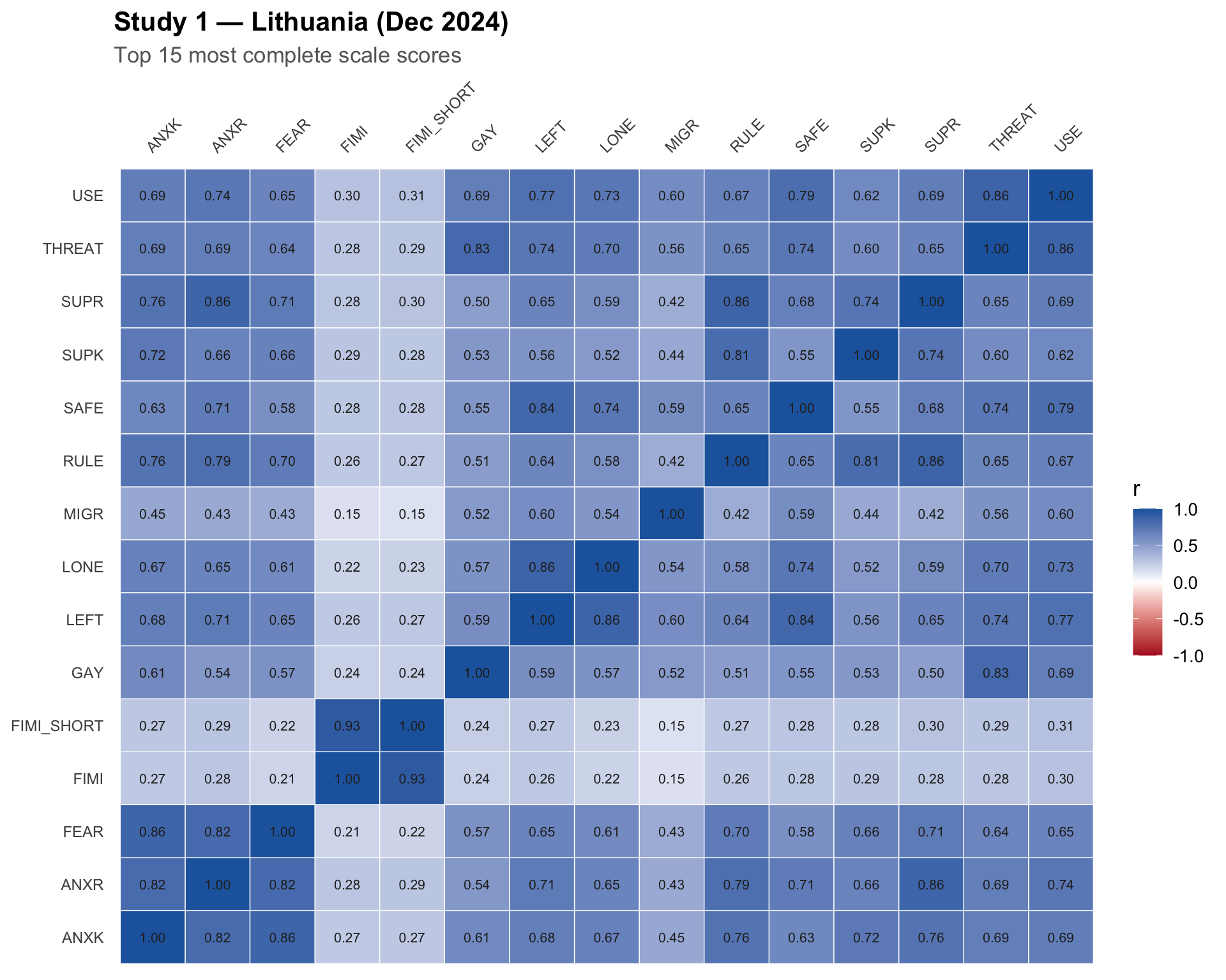
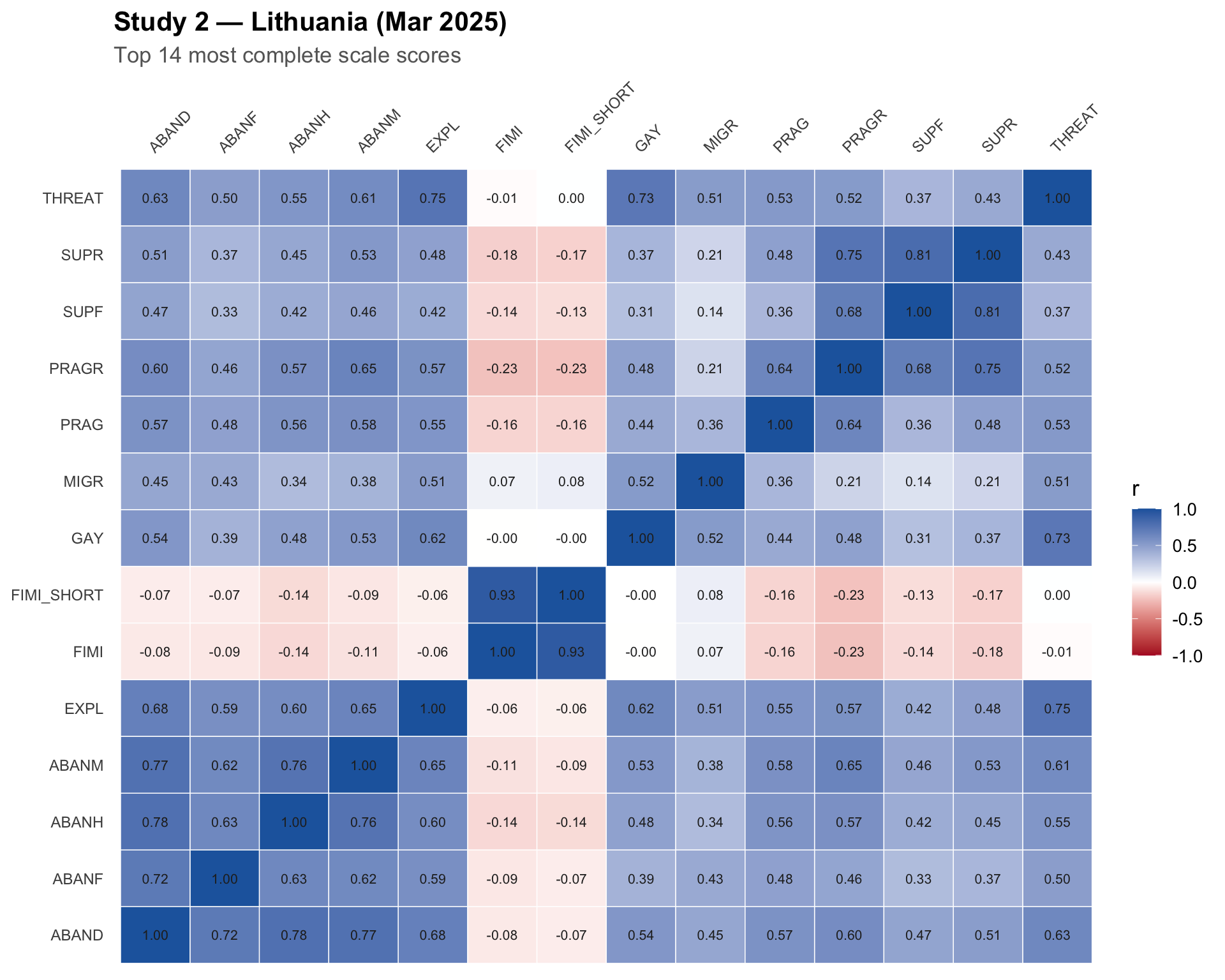
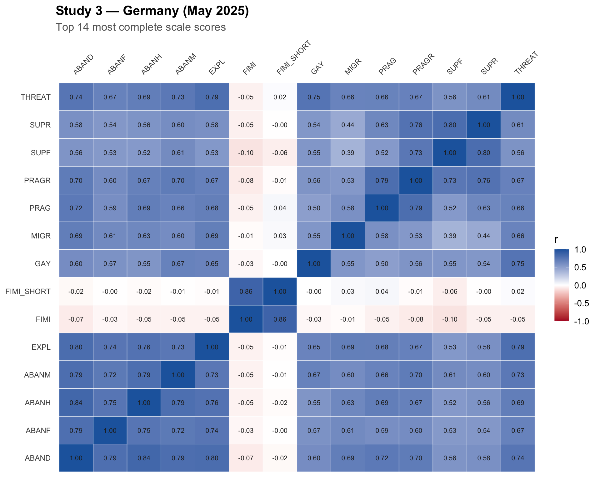
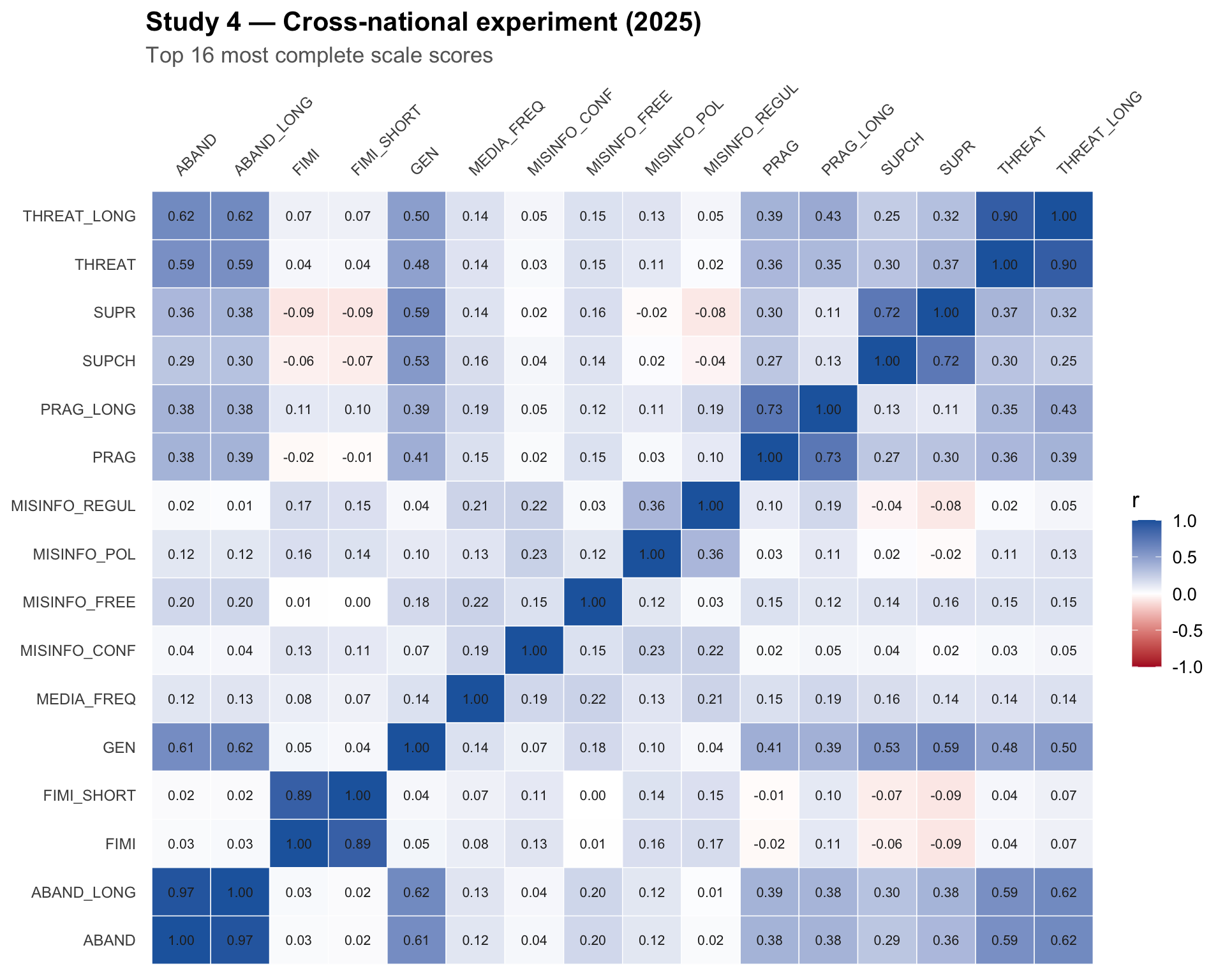
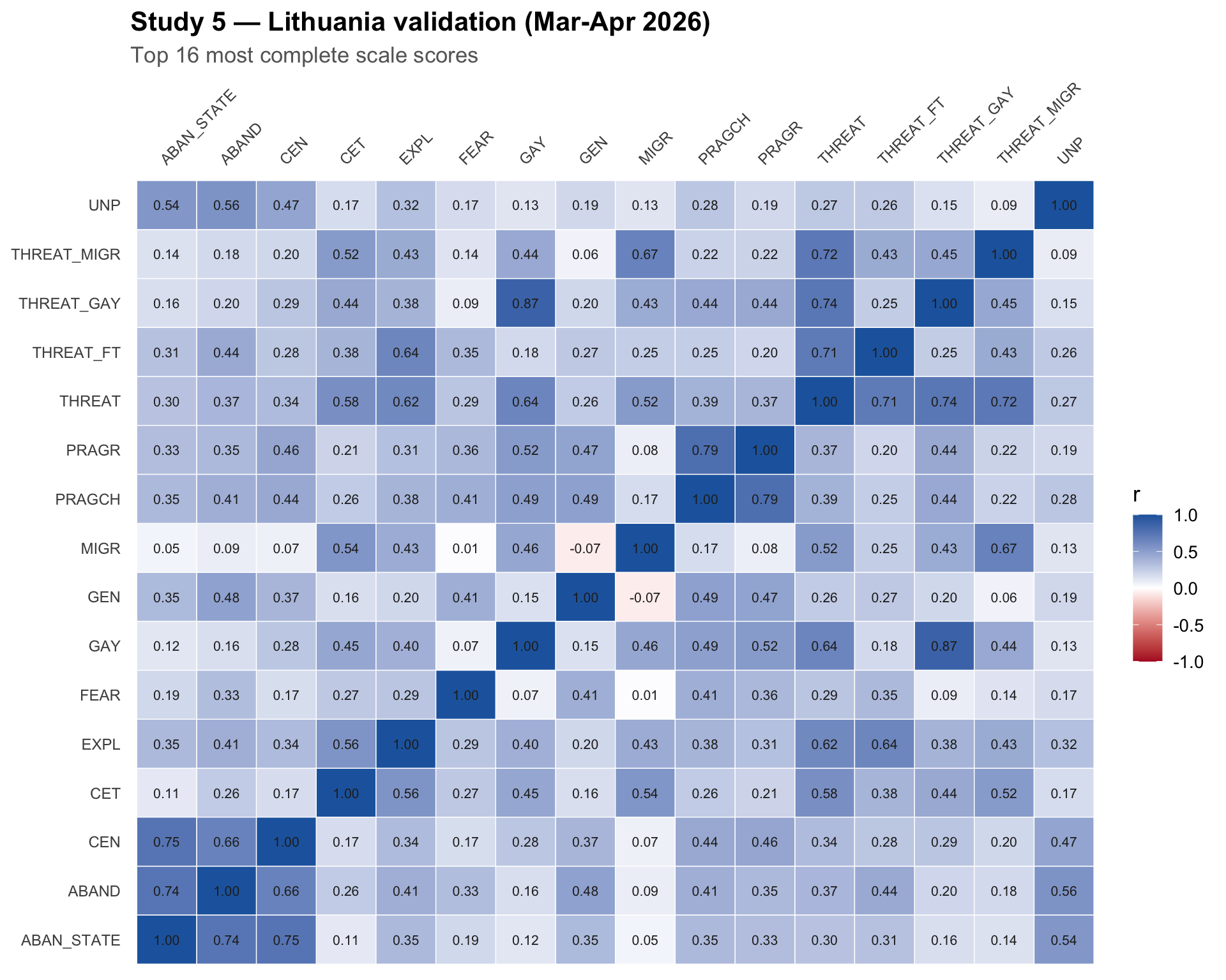
The per-study heatmap caps at the 16 most complete scales so dense studies (S4/S5) remain readable. Cells show Pearson r computed with pairwise complete observations; the numeric annotation makes it easy to lift a value into the manuscript without reading off the colour bar.

Study 1 — Lithuania (Dec 2024)

- Maximum absolute inter-scale correlation in this study: 0.93. ### Study 2 — Lithuania (Mar 2025) - Maximum absolute inter-scale correlation in this study: 0.93. ### Study 3 — Germany (May 2025) - Maximum absolute inter-scale correlation in this study: 0.86. ### Study 4 — Cross-national experiment (2025) - Maximum absolute inter-scale correlation in this study: 0.97. ### Study 5 — Lithuania validation (Mar-Apr 2026) - Maximum absolute inter-scale correlation in this study: 0.96.
Inter-scale correlation tables (APA-style)

For each study we also produce a long-format pairwise correlation table with sample sizes, 95% CIs, two-sided p-values, and APA-style significance stars (* p<.05, ** p<.01, *** p<.001). The table is sorted by absolute r so the strongest associations float to the top.

Study 1 — Lithuania (Dec 2024)

Study 1 — Lithuania (Dec 2024): 25 strongest pairwise inter-scale correlations (full table exported below)
Scale A Scale B n r [sig] 95% CI p
FIMI FIMI_SHORT 681 +0.93*** [+0.92, +0.94] <.001
SUPR RULE 681 +0.86*** [+0.84, +0.88] <.001
LONE LEFT 681 +0.86*** [+0.84, +0.88] <.001
USE THREAT 681 +0.86*** [+0.84, +0.88] <.001
ANXR SUPR 681 +0.86*** [+0.84, +0.88] <.001
ANXK FEAR 681 +0.86*** [+0.84, +0.88] <.001
SAFE LEFT 681 +0.84*** [+0.82, +0.86] <.001
GAY THREAT 681 +0.83*** [+0.80, +0.85] <.001
ANXR FEAR 681 +0.82*** [+0.80, +0.84] <.001
ANXR ANXK 681 +0.82*** [+0.79, +0.84] <.001
SUPK RULE 681 +0.81*** [+0.78, +0.83] <.001
USE SAFE 681 +0.79*** [+0.76, +0.82] <.001
ANXR RULE 681 +0.79*** [+0.76, +0.82] <.001
USE LEFT 681 +0.77*** [+0.74, +0.80] <.001
ANXK SUPR 681 +0.76*** [+0.72, +0.79] <.001
ANXK RULE 681 +0.76*** [+0.72, +0.79] <.001
SUPR SUPK 681 +0.74*** [+0.71, +0.78] <.001
LONE SAFE 681 +0.74*** [+0.70, +0.77] <.001
USE ANXR 681 +0.74*** [+0.70, +0.77] <.001
THREAT LEFT 681 +0.74*** [+0.70, +0.77] <.001
THREAT SAFE 681 +0.74*** [+0.70, +0.77] <.001
USE LONE 681 +0.73*** [+0.69, +0.76] <.001
ANXK SUPK 681 +0.72*** [+0.68, +0.76] <.001
FEAR SUPR 681 +0.71*** [+0.68, +0.75] <.001
LEFT ANXR 681 +0.71*** [+0.68, +0.75] <.001

Study 2 — Lithuania (Mar 2025)

Study 2 — Lithuania (Mar 2025): 25 strongest pairwise inter-scale correlations (full table exported below)
Scale A Scale B n r [sig] 95% CI p
FIMI FIMI_SHORT 582 +0.93*** [+0.91, +0.94] <.001
SUPR SUPF 582 +0.81*** [+0.78, +0.83] <.001
ABANH ABAND 582 +0.78*** [+0.74, +0.81] <.001
ABANM ABAND 582 +0.77*** [+0.73, +0.80] <.001
ABANH ABANM 582 +0.76*** [+0.72, +0.79] <.001
PRAGR SUPR 582 +0.75*** [+0.71, +0.78] <.001
EXPL THREAT 582 +0.75*** [+0.71, +0.78] <.001
GAY THREAT 582 +0.73*** [+0.69, +0.76] <.001
ABANF ABAND 582 +0.72*** [+0.68, +0.76] <.001
PRAGR SUPF 582 +0.68*** [+0.64, +0.73] <.001
EXPL ABAND 582 +0.68*** [+0.63, +0.72] <.001
ABANM PRAGR 582 +0.65*** [+0.60, +0.70] <.001
EXPL ABANM 582 +0.65*** [+0.60, +0.69] <.001
PRAGR PRAG 582 +0.64*** [+0.59, +0.68] <.001
ABANF ABANH 582 +0.63*** [+0.58, +0.68] <.001
THREAT ABAND 582 +0.63*** [+0.58, +0.68] <.001
EXPL GAY 582 +0.62*** [+0.57, +0.67] <.001
ABANF ABANM 582 +0.62*** [+0.57, +0.67] <.001
THREAT ABANM 582 +0.61*** [+0.55, +0.66] <.001
ABAND PRAGR 582 +0.60*** [+0.55, +0.65] <.001
EXPL ABANH 582 +0.60*** [+0.54, +0.65] <.001
EXPL ABANF 582 +0.59*** [+0.53, +0.64] <.001
ABANM PRAG 582 +0.58*** [+0.52, +0.63] <.001
ABANH PRAGR 582 +0.57*** [+0.52, +0.63] <.001
EXPL PRAGR 582 +0.57*** [+0.52, +0.63] <.001

Study 3 — Germany (May 2025)

Study 3 — Germany (May 2025): 25 strongest pairwise inter-scale correlations (full table exported below)
Scale A Scale B n r [sig] 95% CI p
FIMI FIMI_SHORT 782 +0.86*** [+0.84, +0.88] <.001
ABANH ABAND 782 +0.84*** [+0.82, +0.86] <.001
EXPL ABAND 782 +0.80*** [+0.78, +0.83] <.001
SUPR SUPF 782 +0.80*** [+0.77, +0.82] <.001
PRAGR PRAG 782 +0.79*** [+0.77, +0.82] <.001
ABANM ABAND 782 +0.79*** [+0.76, +0.82] <.001
EXPL THREAT 782 +0.79*** [+0.76, +0.81] <.001
ABANH ABANM 782 +0.79*** [+0.76, +0.81] <.001
ABANF ABAND 782 +0.79*** [+0.76, +0.81] <.001
PRAGR SUPR 782 +0.76*** [+0.73, +0.79] <.001
EXPL ABANH 782 +0.76*** [+0.73, +0.79] <.001
GAY THREAT 782 +0.75*** [+0.72, +0.78] <.001
ABANF ABANH 782 +0.75*** [+0.71, +0.78] <.001
THREAT ABAND 782 +0.74*** [+0.71, +0.77] <.001
EXPL ABANF 782 +0.74*** [+0.71, +0.77] <.001
EXPL ABANM 782 +0.73*** [+0.70, +0.76] <.001
PRAGR SUPF 782 +0.73*** [+0.70, +0.76] <.001
THREAT ABANM 782 +0.73*** [+0.69, +0.76] <.001
ABANF ABANM 782 +0.72*** [+0.69, +0.75] <.001
ABAND PRAG 782 +0.72*** [+0.68, +0.75] <.001
ABAND PRAGR 782 +0.70*** [+0.67, +0.74] <.001
ABANM PRAGR 782 +0.70*** [+0.67, +0.74] <.001
MIGR ABAND 782 +0.69*** [+0.65, +0.73] <.001
THREAT ABANH 782 +0.69*** [+0.65, +0.72] <.001
ABANH PRAG 782 +0.69*** [+0.65, +0.72] <.001

Study 4 — Cross-national experiment (2025)

Study 4 — Cross-national experiment (2025): 25 strongest pairwise inter-scale correlations (full table exported below)
Scale A Scale B n r [sig] 95% CI p
ABAND ABAND_LONG 8040 +0.97*** [+0.97, +0.97] <.001
THREAT THREAT_LONG 8040 +0.90*** [+0.90, +0.91] <.001
FIMI FIMI_SHORT 8040 +0.89*** [+0.89, +0.89] <.001
PRAG PRAG_LONG 8040 +0.73*** [+0.72, +0.74] <.001
SUPR SUPCH 8040 +0.72*** [+0.71, +0.73] <.001
THREAT_LONG ABAND 8040 +0.62*** [+0.61, +0.63] <.001
GEN ABAND_LONG 8040 +0.62*** [+0.61, +0.63] <.001
THREAT_LONG ABAND_LONG 8040 +0.62*** [+0.61, +0.63] <.001
GEN ABAND 8040 +0.61*** [+0.59, +0.62] <.001
MISINFO_SRC MISINFO_FOREIGN 8040 +0.59*** [+0.58, +0.60] <.001
GEN SUPR 8040 +0.59*** [+0.57, +0.60] <.001
THREAT ABAND_LONG 8040 +0.59*** [+0.57, +0.60] <.001
THREAT ABAND 8040 +0.59*** [+0.57, +0.60] <.001
GEN SUPCH 8040 +0.53*** [+0.51, +0.54] <.001
GEN THREAT_LONG 8040 +0.50*** [+0.48, +0.52] <.001
MISINFO_IMPACT MISINFO_RESP 8040 +0.49*** [+0.47, +0.50] <.001
INST_TRUST POL_EFF_EXT 8040 +0.49*** [+0.47, +0.50] <.001
GEN THREAT 8040 +0.48*** [+0.46, +0.50] <.001
SOC_TRUST INST_TRUST 8040 +0.46*** [+0.45, +0.48] <.001
INST_TRUST EU_SUPPORT 8040 +0.46*** [+0.44, +0.47] <.001
POL_INTEREST POL_EFF_INT 8040 -0.44*** [-0.46, -0.42] <.001
POL_EFF_EXT POL_EFF_INT 8040 +0.44*** [+0.42, +0.45] <.001
MISINFO_RESP DEM_IMPORT 8040 +0.43*** [+0.42, +0.45] <.001
THREAT_LONG PRAG_LONG 8040 +0.43*** [+0.41, +0.45] <.001
INST_TRUST LIFE_SAT 8040 +0.42*** [+0.40, +0.44] <.001

Study 5 — Lithuania validation (Mar-Apr 2026)

Study 5 — Lithuania validation (Mar-Apr 2026): 25 strongest pairwise inter-scale correlations (full table exported below)
Scale A Scale B n r [sig] 95% CI p
ITT_LGBT ITT_LGBT_SYM 248 +0.96*** [+0.94, +0.97] <.001
ITT_IMI ITT_IMI_SYM 248 +0.92*** [+0.90, +0.94] <.001
ITT_IMI ITT_IMI_REAL 248 +0.92*** [+0.90, +0.94] <.001
ITT_LGBT ITT_LGBT_REAL 248 +0.91*** [+0.89, +0.93] <.001
GAY ITT_LGBT 248 +0.90*** [+0.87, +0.92] <.001
GAY ITT_LGBT_SYM 248 +0.88*** [+0.84, +0.90] <.001
THREAT_GAY GAY 248 +0.87*** [+0.84, +0.90] <.001
THREAT_GAY ITT_LGBT 248 +0.85*** [+0.81, +0.88] <.001
THREAT_GAY ITT_LGBT_SYM 248 +0.83*** [+0.79, +0.87] <.001
GAY ITT_LGBT_REAL 248 +0.79*** [+0.74, +0.83] <.001
PRAGR PRAGCH 248 +0.79*** [+0.74, +0.83] <.001
SUP_GEN SUPR 248 +0.77*** [+0.72, +0.82] <.001
PRAGR SUPR 248 +0.77*** [+0.71, +0.81] <.001
ITT_LGBT_SYM ITT_LGBT_REAL 248 +0.75*** [+0.69, +0.80] <.001
ABAN_STATE CEN 248 +0.75*** [+0.69, +0.80] <.001
MIGR ITT_IMI 248 +0.75*** [+0.69, +0.80] <.001
MIGR ITT_IMI_SYM 248 +0.75*** [+0.69, +0.80] <.001
ABAND ABAN_STATE 248 +0.74*** [+0.68, +0.80] <.001
THREAT_GAY ITT_LGBT_REAL 248 +0.74*** [+0.67, +0.79] <.001
THREAT THREAT_GAY 248 +0.74*** [+0.67, +0.79] <.001
THREAT THREAT_MIGR 248 +0.72*** [+0.66, +0.78] <.001
THREAT THREAT_FT 248 +0.71*** [+0.64, +0.77] <.001
SUP_GEN SUPCH 248 +0.71*** [+0.64, +0.76] <.001
TRUST_EU TRUST_UN 248 +0.70*** [+0.63, +0.76] <.001
SUP_GEN FEEL_CH 247 +0.70*** [+0.63, +0.76] <.001

Pairs panels for focal predictor sets

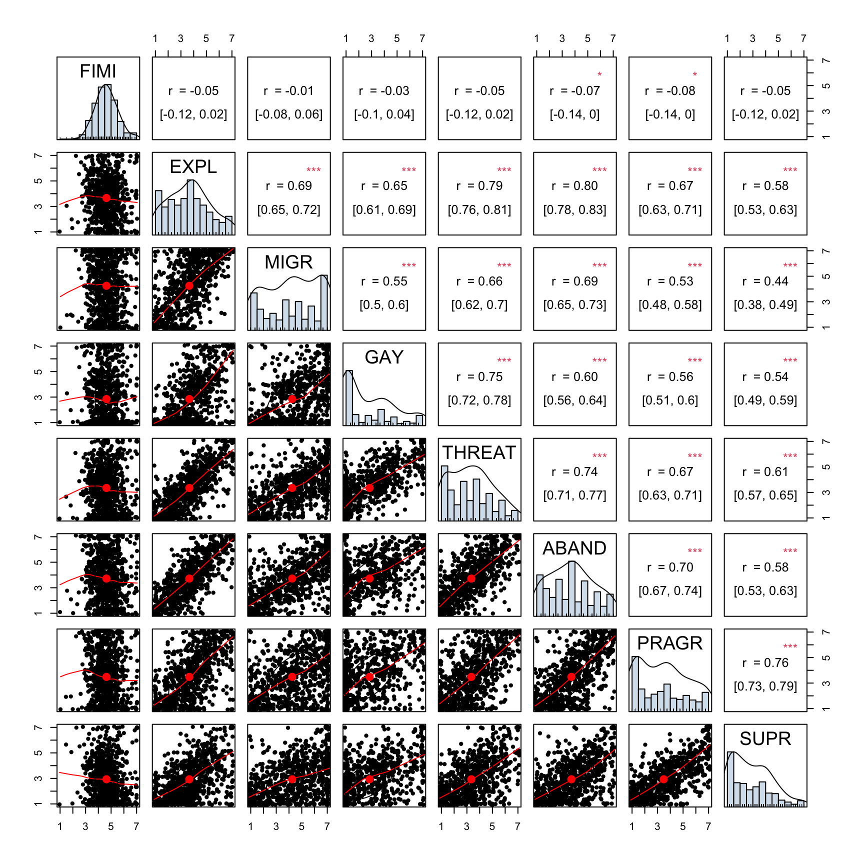
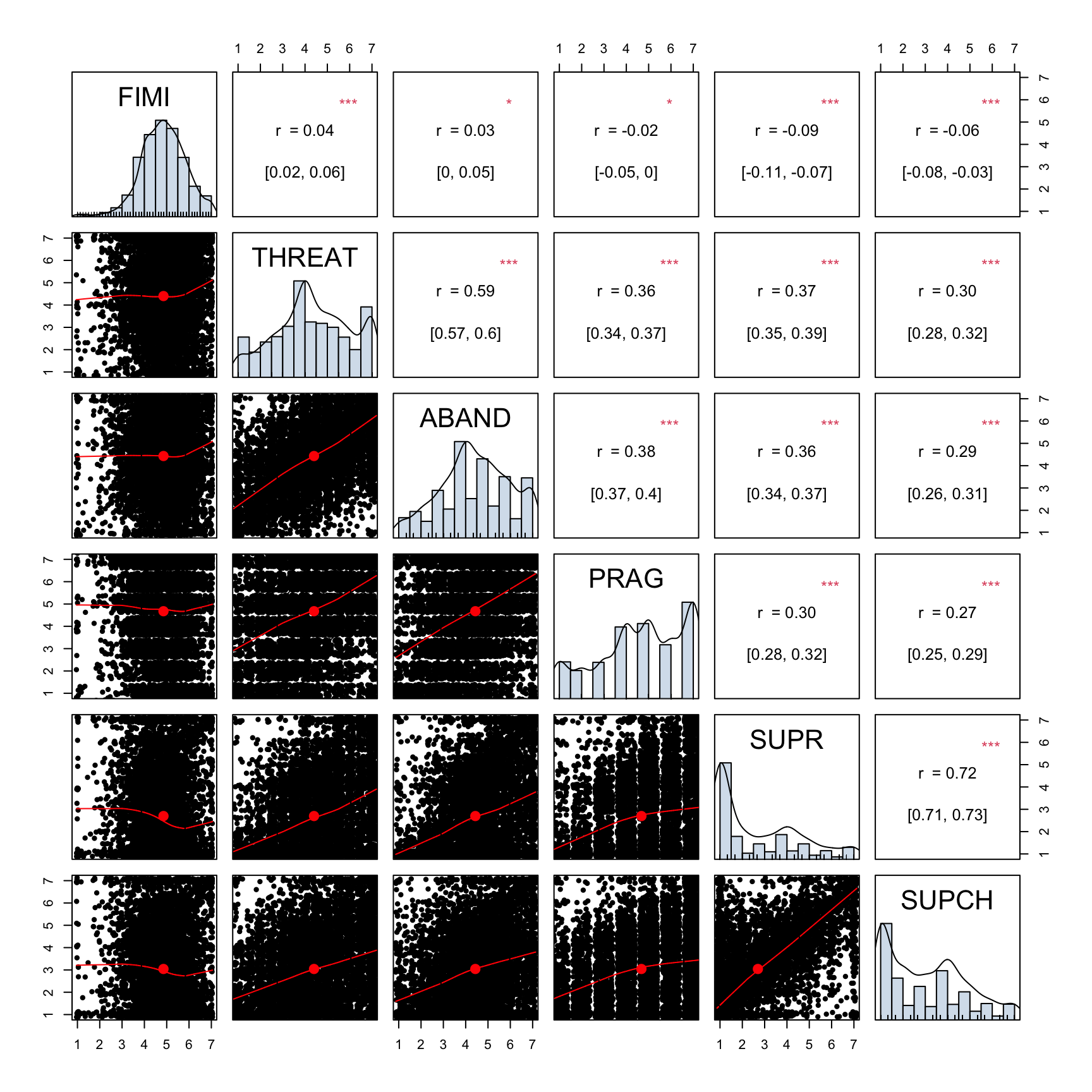
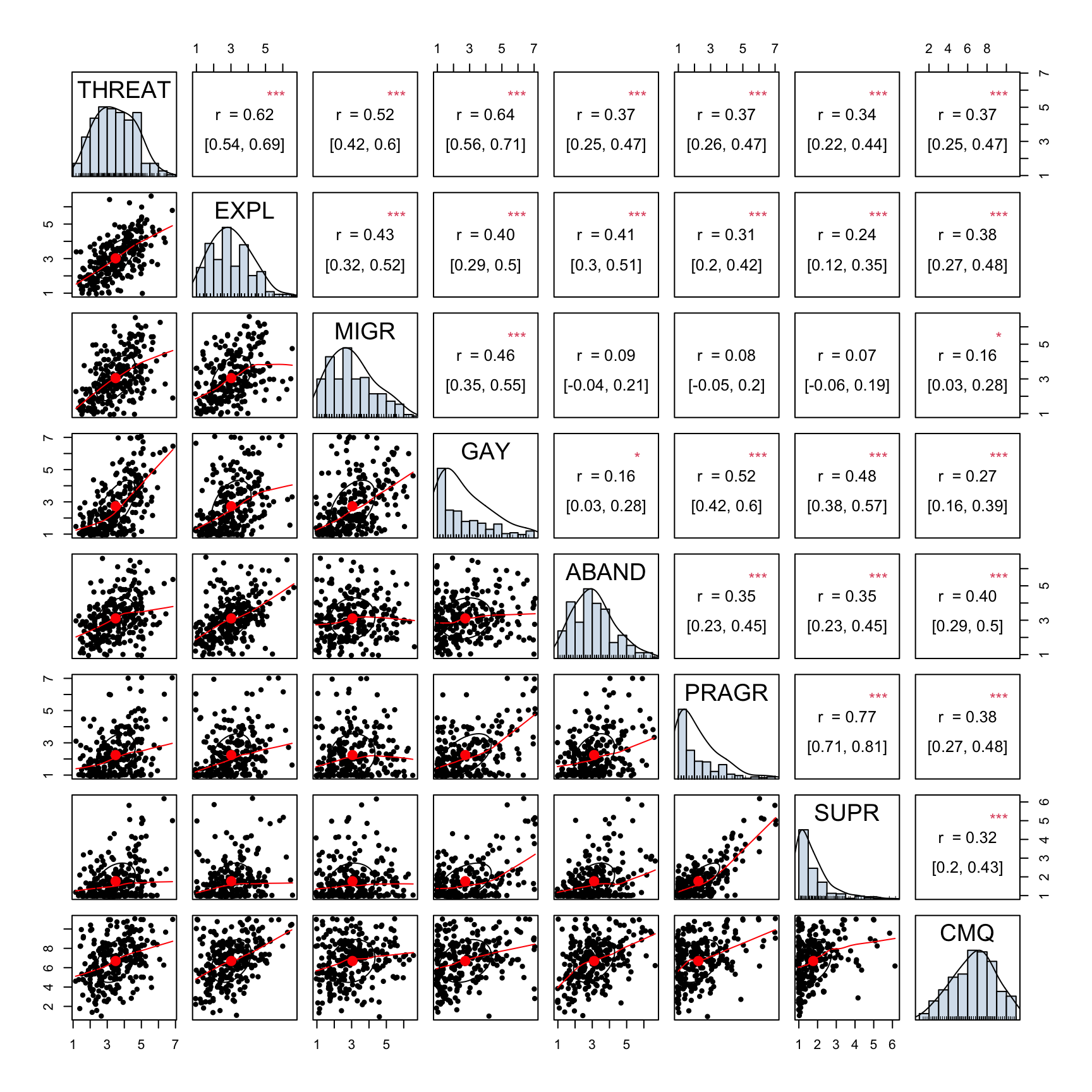
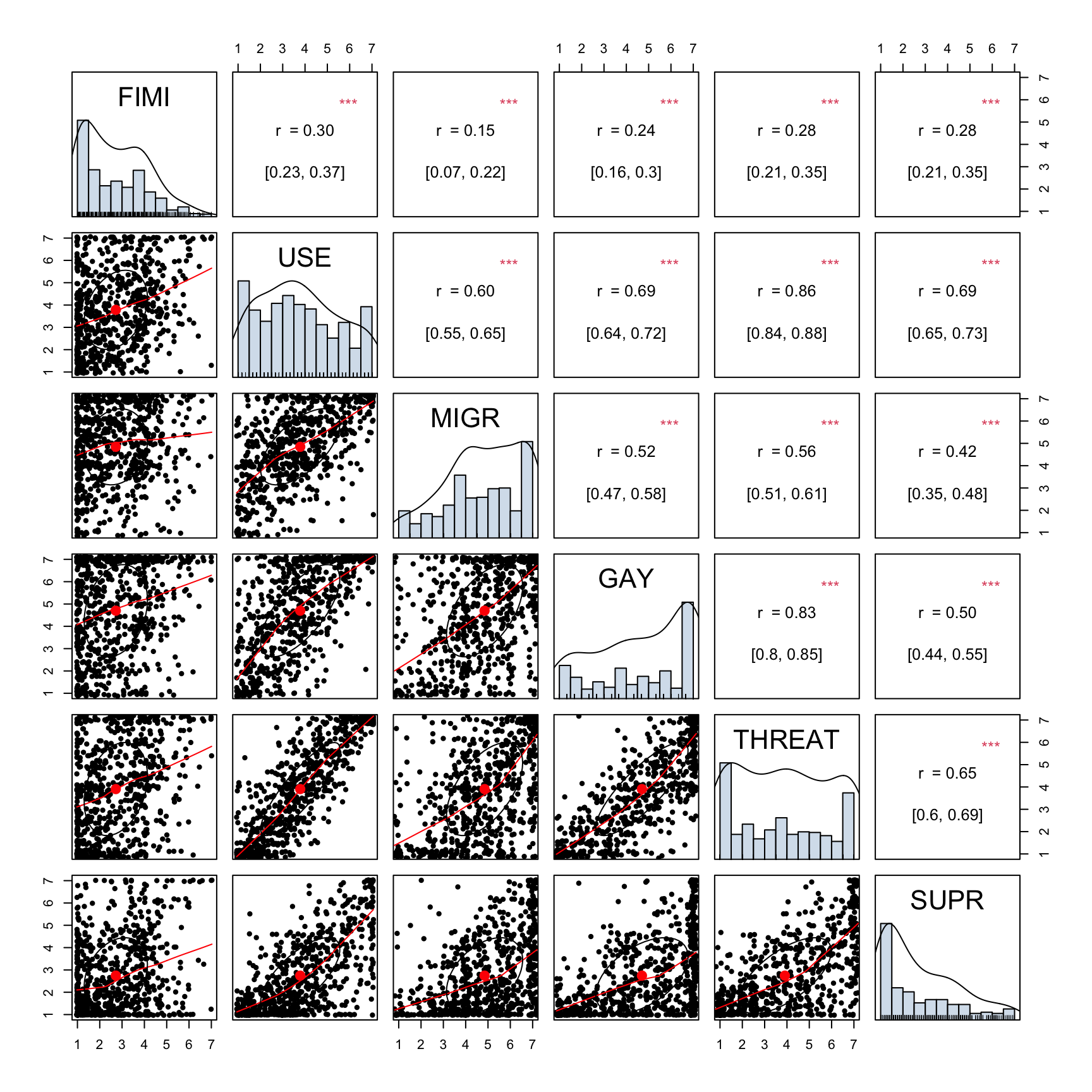
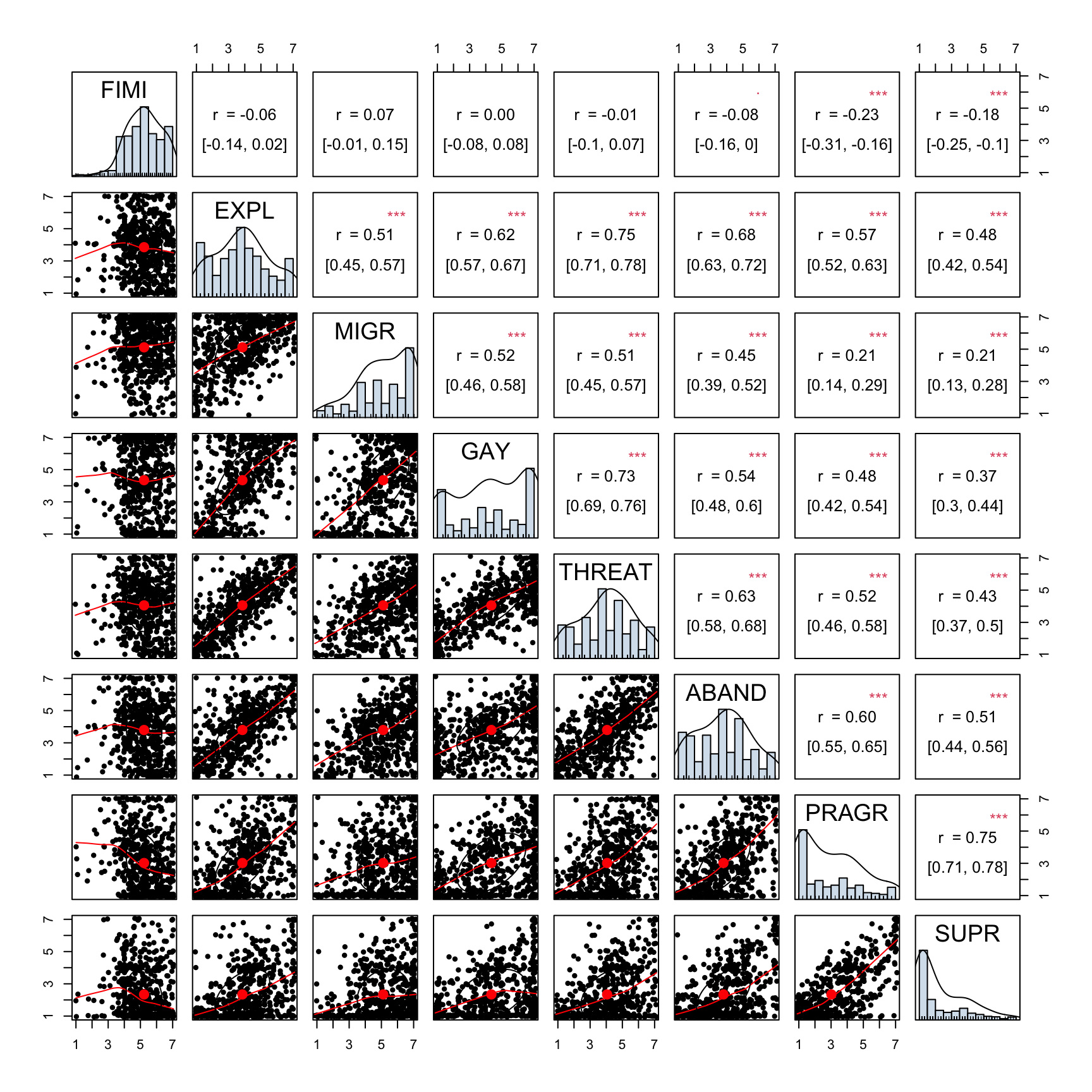
pairs.panels.new() (defined in scripts/functions/fun-panel.R) lays out, for every pair of scales: the bivariate scatter with a lowess + concentration ellipse in the lower triangle, the Pearson r with stars and a 95% CI in the upper triangle, and a histogram + density + rug in the diagonal. We use a study-tailored focal set so the figure stays readable while still covering the constructs that anchor each study’s measurement model.

Study 1 — Lithuania (Dec 2024) — focal predictor pairs

Study 2 — Lithuania (Mar 2025) — focal predictor pairs

Study 3 — Germany (May 2025) — focal predictor pairs

Study 4 — Cross-national experiment (2025) — focal predictor pairs

Study 5 — Lithuania validation (Mar-Apr 2026) — focal predictor pairs

FIMI outcome ←→ predictor diagnostics (S1–S4)

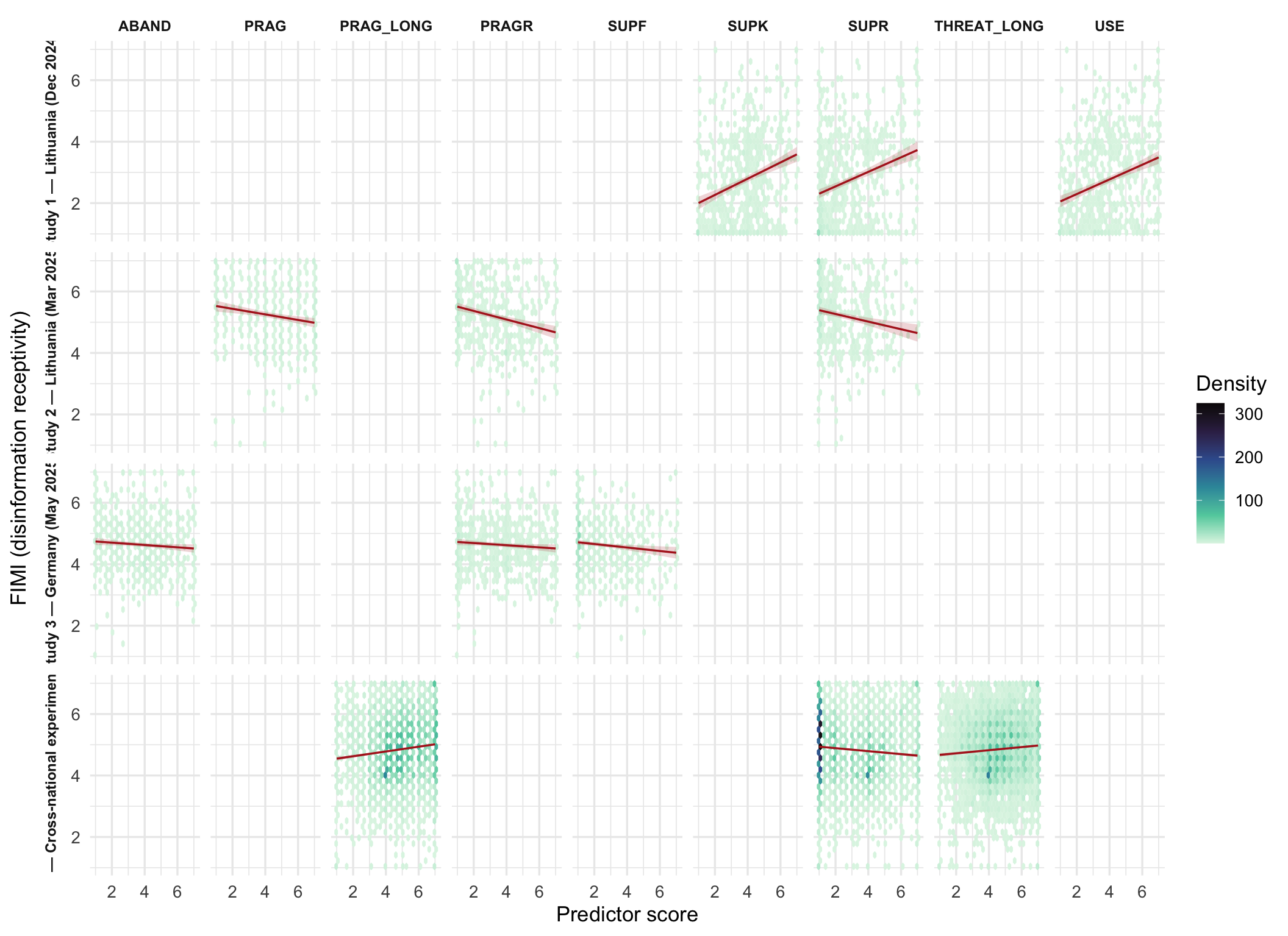
For every study that administered the FIMI battery, we plot the per-respondent FIMI score against the strongest DisInformeter scale predictor correlates and report the rank-ordered correlations. This is the most direct bivariate evidence that the predictor battery moves with the outcome it was designed to predict.

Code
fimi_correlations <- purrr::imap_dfr(scales_data, function(scales_df, study_key) {
  tax <- construct_taxonomy[[study_key]]
  if (is.null(tax) || length(tax$outcome) == 0L) return(tibble())
  predictor_cols <- paste0("scale_", stringr::str_to_lower(tax$predictor))
  predictor_cols <- intersect(predictor_cols, names(scales_df))
  if (length(predictor_cols) == 0L) return(tibble())

  fimi_col <- "scale_fimi"
  if (!fimi_col %in% names(scales_df)) return(tibble())

  purrr::map_dfr(predictor_cols, function(p) {
    x <- suppressWarnings(as.numeric(scales_df[[fimi_col]]))
    y <- suppressWarnings(as.numeric(scales_df[[p]]))
    ok <- is.finite(x) & is.finite(y)
    if (sum(ok) < 4L) {
      return(tibble(predictor = p, n = sum(ok),
                    r = NA_real_, p_value = NA_real_,
                    ci_lower = NA_real_, ci_upper = NA_real_))
    }
    fit <- suppressWarnings(stats::cor.test(x[ok], y[ok]))
    tibble(
      predictor = stringr::str_remove(p, "^scale_") %>% stringr::str_to_upper(),
      n = sum(ok),
      r = unname(fit$estimate),
      p_value = unname(fit$p.value),
      ci_lower = fit$conf.int[1],
      ci_upper = fit$conf.int[2]
    )
  }) %>%
    dplyr::mutate(study_code = study_key)
}) %>%
  dplyr::left_join(study_lookup, by = "study_code") %>%
  dplyr::mutate(label = dplyr::coalesce(label, study_code))

fimi_correlations %>%
  dplyr::filter(!is.na(r)) %>%
  dplyr::arrange(label, dplyr::desc(abs(r))) %>%
  dplyr::mutate(
    r = sprintf("%+.2f", r),
    `95% CI` = sprintf("[%+.2f, %+.2f]", ci_lower, ci_upper),
    p_value = ifelse(p_value < .001, "<.001", sprintf("%.3f", p_value))
  ) %>%
  dplyr::select(label, predictor, n, r, `95% CI`, p_value) %>%
  knitr::kable(
    col.names = c("Study", "Predictor", "n", "r(FIMI)", "95% CI", "p"),
    align = c("l", "l", "r", "r", "r", "r")
  ) %>%
  kableExtra::kable_styling(full_width = FALSE, font_size = 9) %>%
  kableExtra::scroll_box(height = "480px")
FIMI outcome ←→ DisInformeter scale predictor correlations (S1-S4)
Study Predictor n r(FIMI) 95% CI p
Study 1 — Lithuania (Dec 2024) USE 681 +0.30 [+0.23, +0.37] <.001
Study 1 — Lithuania (Dec 2024) SUPK 681 +0.29 [+0.22, +0.35] <.001
Study 1 — Lithuania (Dec 2024) SUPR 681 +0.28 [+0.21, +0.35] <.001
Study 1 — Lithuania (Dec 2024) THREAT 681 +0.28 [+0.21, +0.35] <.001
Study 1 — Lithuania (Dec 2024) ANXR 681 +0.28 [+0.21, +0.35] <.001
Study 1 — Lithuania (Dec 2024) SAFE 681 +0.28 [+0.21, +0.35] <.001
Study 1 — Lithuania (Dec 2024) ANXK 681 +0.27 [+0.19, +0.33] <.001
Study 1 — Lithuania (Dec 2024) RULE 681 +0.26 [+0.19, +0.33] <.001
Study 1 — Lithuania (Dec 2024) LEFT 681 +0.26 [+0.19, +0.33] <.001
Study 1 — Lithuania (Dec 2024) GAY 681 +0.24 [+0.16, +0.30] <.001
Study 1 — Lithuania (Dec 2024) LONE 681 +0.22 [+0.14, +0.29] <.001
Study 1 — Lithuania (Dec 2024) FEAR 681 +0.21 [+0.13, +0.28] <.001
Study 1 — Lithuania (Dec 2024) MIGR 681 +0.15 [+0.07, +0.22] <.001
Study 2 — Lithuania (Mar 2025) PRAGR 582 -0.23 [-0.31, -0.16] <.001
Study 2 — Lithuania (Mar 2025) SUPR 582 -0.18 [-0.25, -0.10] <.001
Study 2 — Lithuania (Mar 2025) PRAG 582 -0.16 [-0.24, -0.08] <.001
Study 2 — Lithuania (Mar 2025) ABANH 582 -0.14 [-0.22, -0.06] <.001
Study 2 — Lithuania (Mar 2025) SUPF 582 -0.14 [-0.22, -0.06] <.001
Study 2 — Lithuania (Mar 2025) ABANM 582 -0.11 [-0.19, -0.03] 0.008
Study 2 — Lithuania (Mar 2025) ABANF 582 -0.09 [-0.17, -0.01] 0.035
Study 2 — Lithuania (Mar 2025) ABAND 582 -0.08 [-0.16, +0.00] 0.058
Study 2 — Lithuania (Mar 2025) MIGR 582 +0.07 [-0.01, +0.15] 0.102
Study 2 — Lithuania (Mar 2025) EXPL 582 -0.06 [-0.14, +0.02] 0.158
Study 2 — Lithuania (Mar 2025) THREAT 582 -0.01 [-0.10, +0.07] 0.730
Study 2 — Lithuania (Mar 2025) GAY 582 -0.00 [-0.08, +0.08] 0.958
Study 3 — Germany (May 2025) SUPF 782 -0.10 [-0.17, -0.03] 0.004
Study 3 — Germany (May 2025) PRAGR 782 -0.08 [-0.14, -0.00] 0.036
Study 3 — Germany (May 2025) ABAND 782 -0.07 [-0.14, -0.00] 0.040
Study 3 — Germany (May 2025) SUPR 782 -0.05 [-0.12, +0.02] 0.138
Study 3 — Germany (May 2025) PRAG 782 -0.05 [-0.12, +0.02] 0.157
Study 3 — Germany (May 2025) THREAT 782 -0.05 [-0.12, +0.02] 0.167
Study 3 — Germany (May 2025) ABANH 782 -0.05 [-0.12, +0.02] 0.179
Study 3 — Germany (May 2025) ABANM 782 -0.05 [-0.12, +0.02] 0.188
Study 3 — Germany (May 2025) EXPL 782 -0.05 [-0.12, +0.02] 0.202
Study 3 — Germany (May 2025) ABANF 782 -0.03 [-0.10, +0.04] 0.385
Study 3 — Germany (May 2025) GAY 782 -0.03 [-0.10, +0.04] 0.466
Study 3 — Germany (May 2025) MIGR 782 -0.01 [-0.08, +0.06] 0.680
Study 4 — Cross-national experiment (2025) PRAG_LONG 8040 +0.11 [+0.09, +0.13] <.001
Study 4 — Cross-national experiment (2025) SUPR 8040 -0.09 [-0.11, -0.07] <.001
Study 4 — Cross-national experiment (2025) THREAT_LONG 8040 +0.07 [+0.05, +0.09] <.001
Study 4 — Cross-national experiment (2025) SUPCH 8040 -0.06 [-0.08, -0.03] <.001
Study 4 — Cross-national experiment (2025) GEN 8040 +0.05 [+0.03, +0.07] <.001
Study 4 — Cross-national experiment (2025) THREAT 8040 +0.04 [+0.02, +0.06] <.001
Study 4 — Cross-national experiment (2025) ABAND_LONG 8040 +0.03 [+0.01, +0.05] 0.012
Study 4 — Cross-national experiment (2025) ABAND 8040 +0.03 [+0.00, +0.05] 0.023
Study 4 — Cross-national experiment (2025) PRAG 8040 -0.02 [-0.05, -0.00] 0.029
Code
top_predictors <- fimi_correlations %>%
  dplyr::filter(!is.na(r)) %>%
  dplyr::group_by(study_code) %>%
  dplyr::slice_max(abs(r), n = 3, with_ties = FALSE) %>%
  dplyr::ungroup()

scatter_long <- top_predictors %>%
  dplyr::rowwise() %>%
  dplyr::mutate(data = list({
    df <- scales_data[[study_code]]
    predictor_col <- paste0("scale_", stringr::str_to_lower(predictor))
    tibble::tibble(
      fimi = suppressWarnings(as.numeric(df[["scale_fimi"]])),
      x = suppressWarnings(as.numeric(df[[predictor_col]]))
    ) %>% dplyr::filter(is.finite(fimi), is.finite(x))
  })) %>%
  dplyr::ungroup() %>%
  tidyr::unnest(data)

ggplot(scatter_long, aes(x = x, y = fimi)) +
  geom_hex(bins = 28, color = NA) +
  geom_smooth(method = "lm", color = "firebrick", fill = "firebrick", alpha = 0.18, linewidth = 0.6) +
  facet_grid(label ~ predictor, scales = "free", switch = "y") +
  scale_fill_viridis_c(option = "mako", direction = -1, name = "Density") +
  labs(x = "Predictor score", y = "FIMI (disinformation receptivity)") +
  theme(
    strip.text = element_text(face = "bold", size = 9),
    strip.placement = "outside",
    legend.position = "right"
  )

FIMI outcome vs the three strongest DisInformeter predictors per study (Studies 1–4). Linear fit + 95% confidence ribbon overlaid on a hex-bin density to avoid overplotting in large samples.
  • Across S1-S4 the top FIMI correlates differ between waves, reflecting that the early Lithuanian formative pool emphasised exploitation / superiority anchors while S2-S4 lean on the harmonised THREAT / ABAND triad.
  • The hex-bin background gives a fair visual weight to dense regions of the scale even in the larger S4 sample, while the linear fit + CI clarifies whether the relationship is monotonic and (where applicable) attenuated by ceiling / floor effects in FIMI.

Export tables and figures

Cross-study highlights

  • Reliability remains stable at the macro level — the SD of alpha across study × scale rows is 0.16, suggesting the harmonised item sets retain comparable internal consistency despite metric drift between waves.
  • S4 contributes the broadest construct coverage (40 scales), while S5 contributes the deepest external-validation battery (21 validation scales).
  • The FIMI outcome (DV) is reported separately from the DisInformeter scale predictors in every per-study and pooled table. FIMI descriptives are fully harmonised across S1-S4 (full and short batteries); S5 is transparently treated as non-FIMI by design.
  • The FIMI ←→ predictor correlations confirm a non-trivial, multi-construct association pattern in every wave — supporting the move to structural-equation models in 03-models/ over univariate inference.

Reproducibility notes

  • Data inputs: data/wrangled_data/study[1-5]_{items,scales}.parquet, scale_blueprints.rds, construct_taxonomy.rds.
  • Helper functions: scripts/functions/descriptives_helpers.R and scripts/functions/fun-panel.R.
  • Cache key: invalidated automatically when any input parquet, the construct taxonomy, the helper scripts, or renv.lock changes.
  • Last rendered: 2026-05-26 11:08:28 CEST.