Predictors, civic anchors & the nomological network

What receptivity domains relate to FIMI detection, how they connect to civic life, and how the whole construct field hangs together

How to read the relationships

This page reports associations between receptivity domains and FIMI detection, the domains’ relationships to civic anchors, and the full nomological network. Two conventions:

• For predictor → detection paths, positive = better detection (the domain travels with recognising manipulation) and negative = a detection blind spot. These are cross-sectional associations, not causal effects (Shadish et al., 2002).
• The headline relationships come from a multilevel Bayesian model (BRMS) of the S4 multinational data; cross-study paths come from the canonical higher-order composite SEM. The heavy estimation is documented on the academic site and in Reproducibility & methods; here we embed the print-ready results and the code that drew them.

The most policy-relevant result: domain meaning changes by source and country

The key finding is not only that countries differ in overall detection — it is that the same receptivity domain can be associated with better detection in one source context and weaker detection in another.

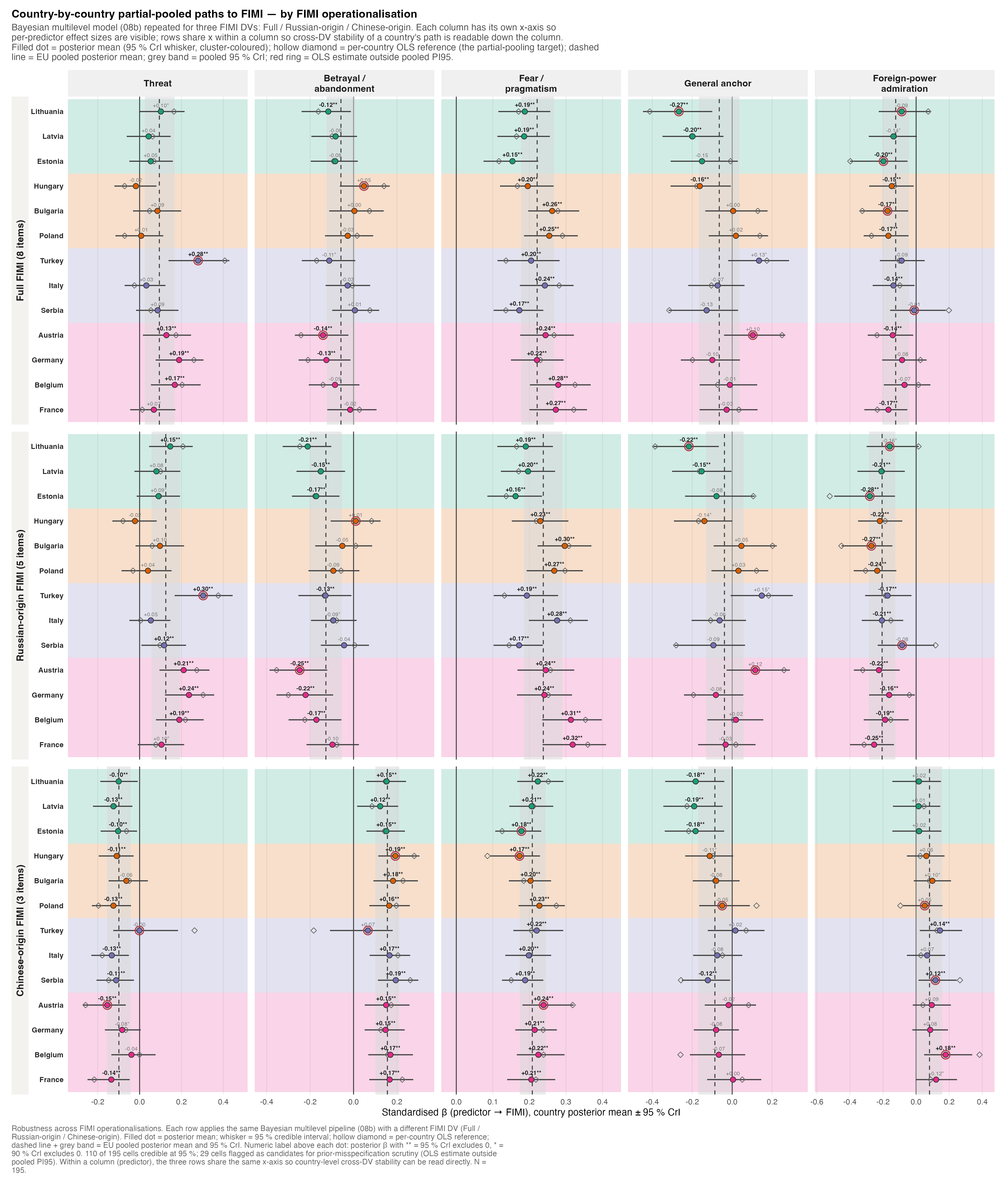
• Fear / Pragmatism is the one consistently protective domain. Respondents more wary of hostile foreign actors detect FIMI better across the board: Full FIMI (= .22) (95% CrI [.18, .27]), Russian-origin (= .24) ([.18, .29]), Chinese-origin (= .21) ([.17, .24]).
• Threat reverses by source: better Russian-origin detection but worse Chinese-origin detection. Betrayal / Abandonment shows the opposite pattern.
• Foreign-Power Admiration is most clearly linked to poorer Russian-origin detection; its Chinese-origin pattern is weaker and less uniform.
• The General Anchor flips by country: negatively associated with detection in some (e.g. Lithuania, Latvia, Hungary, Serbia, depending on variant), but positive for Russian-origin FIMI in Turkey and Austria.

Figure 1: Country predictor → detection paths by FIMI operationalisation (Full, Russian-origin, Chinese-origin), from the S4 multilevel Bayesian model. Positive = better detection; negative = a detection blind spot. The figure shows why source-specific paths must not be collapsed.

ImportantPolicy reading

Do not collapse these paths into a single “FIMI vulnerability” score. The same public attitude can be associated with better detection for one source and worse for another. Monitoring, prebunking, and media-literacy work should report at least three layers together: the country’s domain profile, Full FIMI detection, and source-specific detection paths.

scripts/policy_report/F-22d_country_forest_brms_fimi_variants.R

#!/usr/bin/env Rscript
#' F-22d — Country × predictor forest plot across FIMI operationalisations.
#'
#' Robustness companion to F-22b. Same Bayesian multilevel partial-pooling
#' model (08b), but fitted three times against the three FIMI DV variants:
#'
#'   ROW 1 — Full FIMI (8 items, the primary DV used in F-22b)
#'   ROW 2 — Russian-origin FIMI (5 items)
#'   ROW 3 — Chinese-origin FIMI (3 items)
#'
#' Within a column (predictor), the three rows are directly comparable —
#' they share the same x-axis range. Cross-row stability of the country
#' posterior pattern indicates the country-level path is robust to which
#' subset of FIMI items defines the outcome; cross-row divergence flags
#' a predictor whose path depends on the FIMI variant.
#'
#' Source CSVs (produced by 08b run once per variant):
#'   outputs/policy_report/tables/s4_country_predictor_paths_brms_full.csv
#'   outputs/policy_report/tables/s4_country_predictor_paths_brms_russian.csv
#'   outputs/policy_report/tables/s4_country_predictor_paths_brms_chinese.csv
#'   outputs/policy_report/tables/s4_country_predictor_pooled_brms_{full,russian,chinese}.csv
#'
#' Output:
#'   outputs/policy_report/figures/F-22d_country_forest_brms_fimi_variants.{png,pdf,rds}

suppressPackageStartupMessages({
  library(ggplot2)
  library(dplyr)
  library(readr)
  library(forcats)
  library(patchwork)
  library(here)
})

source(here::here("scripts", "policy_report", "_theme.R"))

SCRIPT_ID  <- "F-22d_country_forest_brms_fimi_variants"
OUT_BASE   <- file.path(POLICY_REPORT_FIG_DIR, SCRIPT_ID)

set.seed(42)

VARIANTS <- c(
  "full"    = "Full FIMI (8 items)",
  "russian" = "Russian-origin FIMI (5 items)",
  "chinese" = "Chinese-origin FIMI (3 items)"
)

# ---- Read + bind all three variants ---------------------------------------

read_variant <- function(slug, label) {
  paths_csv <- here::here(
    "outputs", "policy_report", "tables",
    sprintf("s4_country_predictor_paths_brms_%s.csv", slug)
  )
  pooled_csv <- here::here(
    "outputs", "policy_report", "tables",
    sprintf("s4_country_predictor_pooled_brms_%s.csv", slug)
  )
  if (!file.exists(paths_csv) || !file.exists(pooled_csv)) {
    stop(sprintf(paste0("F-22d: required input(s) missing for variant '%s'.\n",
                        "  expected: %s\n  expected: %s\n",
                        "Run main_08b_all_variants() in ",
                        "R/policy_report/08b_country_predictor_brms.R first."),
                 slug, paths_csv, pooled_csv), call. = FALSE)
  }
  list(
    paths  = readr::read_csv(paths_csv,  show_col_types = FALSE) |>
              dplyr::mutate(fimi_variant_slug  = slug,
                            fimi_variant_label = label),
    pooled = readr::read_csv(pooled_csv, show_col_types = FALSE) |>
              dplyr::mutate(fimi_variant_slug  = slug,
                            fimi_variant_label = label)
  )
}

variant_data <- purrr::map2(names(VARIANTS), unname(VARIANTS), read_variant)
dat <- dplyr::bind_rows(lapply(variant_data, `[[`, "paths"))
pooled <- dplyr::bind_rows(lapply(variant_data, `[[`, "pooled"))

if (nrow(dat) == 0L || nrow(pooled) == 0L) {
  stop("F-22d: combined per-variant inputs returned zero rows.",
       call. = FALSE)
}

# ---- Country + predictor ordering -----------------------------------------

PREDICTOR_ORDER <- c("THREAT", "ABAND", "FEAR", "GEN", "SUPF")
PREDICTOR_LBL <- c(
  THREAT = "Threat",
  ABAND  = "Betrayal /\nabandonment",
  FEAR   = "Fear /\npragmatism",
  GEN    = "General anchor",
  SUPF   = "Foreign-power\nadmiration"
)
CLUSTER_ORDER <- c("Baltic", "Central-East", "Southern", "Western")

# Country order — by regional cluster then average |posterior| in the Full
# FIMI variant (so the row order is anchored to the primary DV and the
# robustness rows below are visually comparable line-by-line).
country_avg <- dat |>
  dplyr::filter(fimi_variant_slug == "full",
                predictor %in% PREDICTOR_ORDER) |>
  dplyr::group_by(country_iso3, country_name, cluster) |>
  dplyr::summarise(mean_abs = mean(abs(posterior_mean), na.rm = TRUE),
                   .groups = "drop") |>
  dplyr::mutate(cluster = factor(cluster, levels = CLUSTER_ORDER)) |>
  dplyr::arrange(dplyr::desc(cluster), mean_abs)
country_order <- country_avg$country_name

sig_marker <- function(sig_95, sig_90) {
  dplyr::case_when(
    sig_95           ~ "**",
    sig_90 & !sig_95 ~ "*",
    TRUE             ~ ""
  )
}

dat <- dat |>
  dplyr::filter(predictor %in% PREDICTOR_ORDER) |>
  dplyr::mutate(
    predictor       = factor(PREDICTOR_LBL[predictor],
                              levels = PREDICTOR_LBL[PREDICTOR_ORDER]),
    country_name    = factor(country_name, levels = country_order),
    cluster         = factor(cluster, levels = CLUSTER_ORDER),
    fimi_variant_label = factor(fimi_variant_label, levels = unname(VARIANTS)),
    asterisk        = sig_marker(sig_95, sig_90),
    label_text      = sprintf("%+.2f%s", posterior_mean, asterisk),
    flagged_prior   = !in_eu_pi95
  )

pooled <- pooled |>
  dplyr::filter(predictor %in% PREDICTOR_ORDER) |>
  dplyr::mutate(predictor = factor(PREDICTOR_LBL[predictor],
                                    levels = PREDICTOR_LBL[PREDICTOR_ORDER]),
                fimi_variant_label = factor(fimi_variant_label,
                                             levels = unname(VARIANTS)))

# ---- Cluster bands + palette ----------------------------------------------

cluster_pal <- setNames(
  policy_report_palette("categorical", n = 4L),
  CLUSTER_ORDER
)
dat <- dat |>
  dplyr::mutate(cluster_fill = cluster_pal[as.character(cluster)])

band_alpha_pal <- setNames(
  paste0(cluster_pal, "33"),  # ~20 % alpha
  CLUSTER_ORDER
)
cluster_bands <- country_avg |>
  dplyr::mutate(y_idx = match(country_name, country_order)) |>
  dplyr::group_by(cluster) |>
  dplyr::summarise(ymin = min(y_idx) - 0.5,
                   ymax = max(y_idx) + 0.5,
                   y_mid = (min(y_idx) + max(y_idx)) / 2,
                   .groups = "drop") |>
  dplyr::mutate(band_fill = band_alpha_pal[as.character(cluster)],
                cluster_label = as.character(cluster))

# ---- Build the 3×5 forest plot --------------------------------------------

n_sig    <- sum(dat$sig_95, na.rm = TRUE)
n_total  <- nrow(dat)
n_flagged <- sum(dat$flagged_prior, na.rm = TRUE)

caption <- policy_report_caption(
  source = "outputs/policy_report/tables/s4_country_predictor_paths_brms_{full,russian,chinese}.csv",
  n      = n_total,
  script = paste0(SCRIPT_ID, ".R"),
  prefix = sprintf(paste0(
    "Robustness across FIMI operationalisations. Each row applies the same ",
    "Bayesian multilevel pipeline (08b) with a different FIMI DV (Full / ",
    "Russian-origin / Chinese-origin). Filled dot = posterior mean; whisker ",
    "= 95 %% credible interval; hollow diamond = per-country OLS reference; ",
    "dashed line + grey band = EU pooled posterior mean and 95 %% CrI. ",
    "Numeric label above each dot: posterior β with ** = 95 %% CrI excludes 0, ",
    "* = 90 %% CrI excludes 0. %d of %d cells credible at 95 %%; %d cells ",
    "flagged as candidates for prior-misspecification scrutiny (OLS estimate ",
    "outside pooled PI95). Within a column (predictor), the three rows share ",
    "the same x-axis so country-level cross-DV stability can be read directly."),
    n_sig, n_total, n_flagged),
  width = 145L
)

p_forest <- ggplot2::ggplot(
    dat,
    ggplot2::aes(x = posterior_mean, y = country_name)
  ) +
  # Cluster row bands.
  ggplot2::geom_rect(
    data = cluster_bands,
    ggplot2::aes(ymin = ymin, ymax = ymax,
                 xmin = -Inf, xmax = Inf,
                 fill = band_fill),
    inherit.aes = FALSE,
    colour = NA
  ) +
  ggplot2::scale_fill_identity() +
  # Vertical zero reference.
  ggplot2::geom_vline(xintercept = 0, colour = "grey25",
                      linewidth = 0.45) +
  # EU pooled CrI band per facet (per row × column).
  ggplot2::geom_rect(
    data = pooled,
    ggplot2::aes(xmin = eu_q025, xmax = eu_q975,
                 ymin = -Inf,    ymax = Inf),
    inherit.aes = FALSE,
    fill = "grey85", colour = NA, alpha = 0.55
  ) +
  # EU pooled posterior mean (dashed vertical).
  ggplot2::geom_vline(
    data = pooled,
    ggplot2::aes(xintercept = eu_pooled_mean),
    colour = "grey25", linewidth = 0.5, linetype = "dashed"
  ) +
  # Country 95 % CrI whisker.
  ggplot2::geom_errorbarh(
    ggplot2::aes(xmin = q025, xmax = q975),
    height = 0, linewidth = 0.55, colour = "grey25"
  ) +
  # ML reference (hollow diamond).
  ggplot2::geom_point(
    ggplot2::aes(x = ml_estimate, y = country_name),
    shape = 5, size = 1.6, stroke = 0.5, colour = "grey40"
  ) +
  # Country posterior mean (filled dot, cluster colour).
  ggplot2::geom_point(
    ggplot2::aes(fill = cluster_fill),
    shape = 21, size = 2.3, stroke = 0.5, colour = "grey20"
  ) +
  # Red ring on prior-misspecification flagged cells.
  ggplot2::geom_point(
    data = dat |> dplyr::filter(flagged_prior),
    ggplot2::aes(x = posterior_mean, y = country_name),
    shape = 21, size = 3.6, stroke = 0.8,
    fill = NA, colour = "#B23A48"
  ) +
  # Label above the dot — two layers because ggplot2 has no
  # `scale_fontface_identity`.
  ggplot2::geom_text(
    data = dat |> dplyr::filter(sig_95),
    ggplot2::aes(label = label_text),
    vjust = -1.05, hjust = 0.5,
    size = 2.2, colour = "grey10", fontface = "bold",
    family = .policy_report_resolve_font(POLICY_REPORT_BASE_FONT)
  ) +
  ggplot2::geom_text(
    data = dat |> dplyr::filter(!sig_95),
    ggplot2::aes(label = label_text),
    vjust = -1.05, hjust = 0.5,
    size = 2.0, colour = "grey45", fontface = "plain",
    family = .policy_report_resolve_font(POLICY_REPORT_BASE_FONT)
  ) +
  ggplot2::facet_grid(rows = ggplot2::vars(fimi_variant_label),
                       cols = ggplot2::vars(predictor),
                       scales = "free_x", switch = "y") +
  ggplot2::scale_x_continuous(
    breaks = scales::pretty_breaks(n = 4),
    expand = ggplot2::expansion(mult = c(0.10, 0.10))
  ) +
  ggplot2::labs(
    title    = "Country-by-country partial-pooled paths to FIMI — by FIMI operationalisation",
    subtitle = policy_report_wrap(
      paste0("Bayesian multilevel model (08b) repeated for three FIMI DVs: ",
             "Full / Russian-origin / Chinese-origin. Each column has its ",
             "own x-axis so per-predictor effect sizes are visible; rows ",
             "share x within a column so cross-DV stability of a country's ",
             "path is readable down the column. Filled dot = posterior mean ",
             "(95 % CrI whisker, cluster-coloured); hollow diamond = per-",
             "country OLS reference (the partial-pooling target); dashed ",
             "line = EU pooled posterior mean; grey band = pooled 95 % CrI; ",
             "red ring = OLS estimate outside pooled PI95."),
      width = 145
    ),
    x = "Standardised β (predictor → FIMI), country posterior mean ± 95 % CrI",
    y = NULL,
    caption = caption
  ) +
  theme_policy_report(base_size = 10) +
  ggplot2::theme(
    panel.grid.major.y = ggplot2::element_blank(),
    panel.grid.major.x = ggplot2::element_line(colour = "grey94"),
    strip.text.x       = ggplot2::element_text(face = "bold",
                                                 lineheight = 0.95,
                                                 size = 9.5),
    strip.text.y.left  = ggplot2::element_text(face = "bold",
                                                 angle = 90,
                                                 size  = 10,
                                                 colour = "grey10",
                                                 lineheight = 0.95),
    strip.background.x = ggplot2::element_rect(fill = "grey94", colour = NA),
    strip.background.y = ggplot2::element_rect(fill = "#F4F2EE", colour = NA),
    strip.placement    = "outside",
    panel.spacing.x    = grid::unit(0.5, "lines"),
    panel.spacing.y    = grid::unit(0.5, "lines"),
    axis.text.y        = ggplot2::element_text(size = 7.6,
                                                face = "bold",
                                                colour = "grey15")
  )

# No cluster patchwork strip — across the 3 facet rows it can't align
# cleanly. The cluster grouping is conveyed by (a) the cluster-coloured
# row bands inside every panel, (b) the cluster-coloured posterior dots,
# and (c) the bold country names on the y-axis. We add a small in-panel
# cluster annotation at the left edge of the leftmost column on each row.
cluster_annot <- cluster_bands |>
  dplyr::mutate(
    fimi_variant_label = factor(unname(VARIANTS)[1],
                                 levels = unname(VARIANTS)),
    predictor          = factor(PREDICTOR_LBL[PREDICTOR_ORDER[1L]],
                                 levels = PREDICTOR_LBL[PREDICTOR_ORDER])
  )

p_final <- p_forest

# A3 portrait-ish: tall to fit 3 rows of 13 countries each.
paths <- safe_ggsave_rds(p_final, OUT_BASE,
                         width  = 14.5,
                         height = 17.0,
                         dpi    = 300)

# Cross-variant stability quick summary.
stability <- dat |>
  dplyr::select(country_iso3, predictor, fimi_variant_slug, posterior_mean,
                sig_95) |>
  tidyr::pivot_wider(names_from = fimi_variant_slug,
                      values_from = c(posterior_mean, sig_95))

# How many cells flip sign across variants?
flip_count <- stability |>
  dplyr::mutate(
    sign_full    = sign(posterior_mean_full),
    sign_russian = sign(posterior_mean_russian),
    sign_chinese = sign(posterior_mean_chinese),
    flips = (sign_full != sign_russian) |
            (sign_full != sign_chinese) |
            (sign_russian != sign_chinese)
  ) |>
  dplyr::summarise(n_flip_cells = sum(flips, na.rm = TRUE)) |>
  dplyr::pull(n_flip_cells)

policy_report_log_outputs(
  SCRIPT_ID, paths, input_rows = nrow(dat),
  extra = c(
    sprintf("Variants plotted: %s", paste(names(VARIANTS), collapse = ", ")),
    sprintf("Country × predictor × variant cells: %d", n_total),
    sprintf("Credible (95 %% CrI excludes 0): %d / %d", n_sig, n_total),
    sprintf("Cells flagged (ML outside pooled PI95): %d", n_flagged),
    sprintf("Sign-flip cells (posterior sign differs across variants): %d / 65",
            flip_count)
  )
)

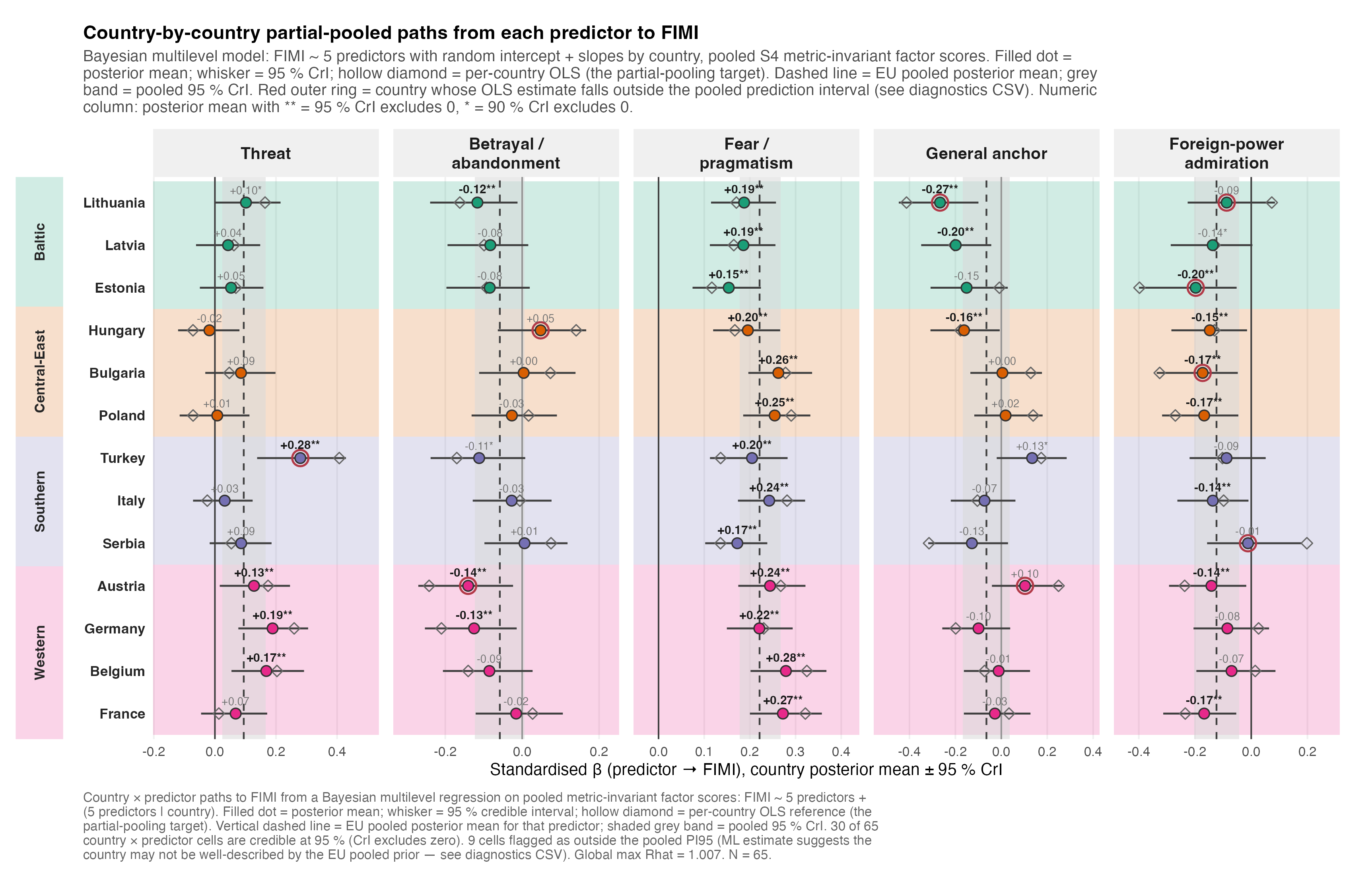
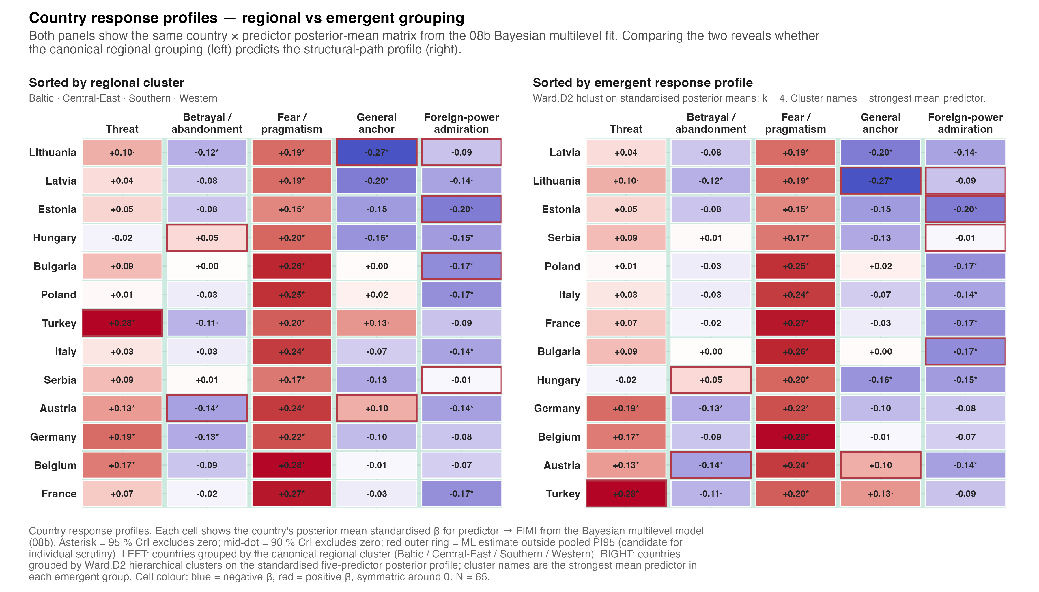
The companion partial-path figures for Full FIMI (point estimates and a path heat-map) are below.

Figure 2: Country partial paths to Full FIMI detection (BRMS).

Figure 3: Country path heat-map for Full FIMI detection (BRMS).

Cross-study predictor paths and explained variance

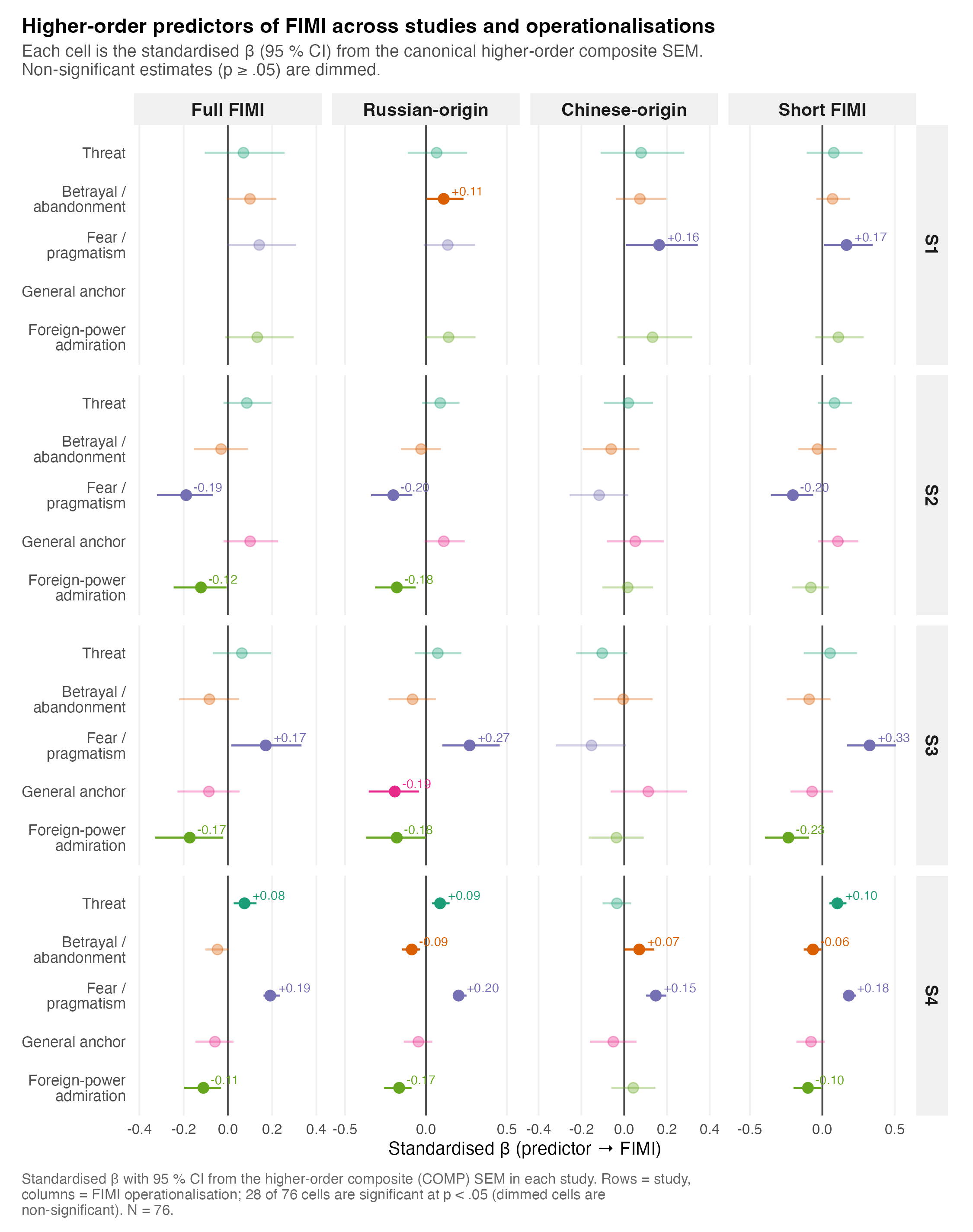
Across studies and FIMI operationalisations, the canonical higher-order composite SEM gives the standardised predictor → FIMI paths (forest plot) and the variance explained (R²). The R² panel provides scale for the predictive models and discourages over-reading individual coefficients.

Figure 4: Cross-study predictor → FIMI forest plot (standardised β, 95% CI). Rows = study; columns = FIMI operationalisation. Non-significant points are dimmed.

Figure 5: Explained variance (R²) by study and FIMI operationalisation.

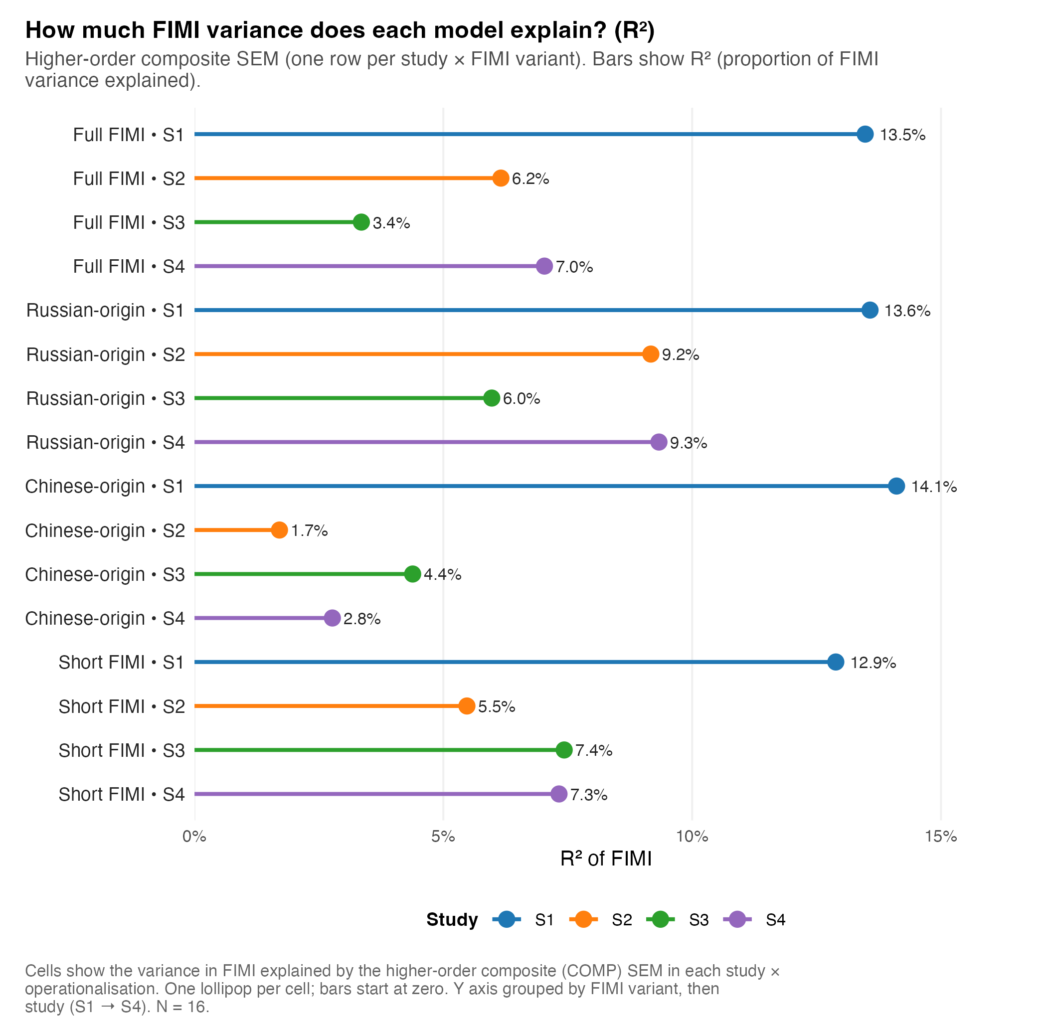
Full structural path estimates (Annex E.1):

Table 1

Annex E.1 — Full structural path estimates
Standardised β coefficients from each higher-order DisInforMeter composite to each FIMI operationalisation. Per-study rows come from the canonical COMP family of prediction models (same filter as F-18); S4 rows reflect the overall structural model. ✓ marks paths with p < .05.
Study	FIMI version	Predictor	β (std)	SE	z	p	CI lower	CI upper	Sig	Block
S1	Chinese FIMI	ABAND	0.073	0.060	1.311	0.1899	−0.039	0.198		Per-study prediction (COMP family)
S1	Chinese FIMI	FEAR	0.163	0.086	2.061	0.0393	0.009	0.344	✓	Per-study prediction (COMP family)
S1	Chinese FIMI	SUPF	0.133	0.089	1.607	0.1080	−0.031	0.318		Per-study prediction (COMP family)
S1	Chinese FIMI	THREAT	0.079	0.100	0.860	0.3898	−0.109	0.281		Per-study prediction (COMP family)
S1	Full FIMI	ABAND	0.100	0.057	1.883	0.0597	−0.004	0.220		Per-study prediction (COMP family)
S1	Full FIMI	FEAR	0.142	0.080	1.916	0.0554	−0.004	0.309		Per-study prediction (COMP family)
S1	Full FIMI	SUPF	0.133	0.079	1.801	0.0717	−0.013	0.298		Per-study prediction (COMP family)
S1	Full FIMI	THREAT	0.071	0.092	0.823	0.4107	−0.105	0.256		Per-study prediction (COMP family)
S1	Russian FIMI	ABAND	0.109	0.058	2.027	0.0426	0.004	0.232	✓	Per-study prediction (COMP family)
S1	Russian FIMI	FEAR	0.134	0.081	1.781	0.0748	−0.014	0.303		Per-study prediction (COMP family)
S1	Russian FIMI	SUPF	0.139	0.080	1.882	0.0598	−0.006	0.306		Per-study prediction (COMP family)
S1	Russian FIMI	THREAT	0.066	0.094	0.754	0.4508	−0.113	0.254		Per-study prediction (COMP family)
S1	Short FIMI	ABAND	0.071	0.060	1.269	0.2043	−0.041	0.192		Per-study prediction (COMP family)
S1	Short FIMI	FEAR	0.167	0.086	2.081	0.0375	0.010	0.348	✓	Per-study prediction (COMP family)
S1	Short FIMI	SUPF	0.111	0.085	1.396	0.1628	−0.048	0.286		Per-study prediction (COMP family)
S1	Short FIMI	THREAT	0.079	0.098	0.863	0.3880	−0.108	0.278		Per-study prediction (COMP family)
S2	Chinese FIMI	ABAND	−0.245	0.160	−1.569	0.1166	−0.563	0.062		Per-study prediction (COMP family)
S2	Chinese FIMI	FEAR	−0.139	0.073	−1.935	0.0530	−0.285	0.002		Per-study prediction (COMP family)
S2	Chinese FIMI	GEN	−0.020	0.121	−0.170	0.8649	−0.257	0.216		Per-study prediction (COMP family)
S2	Chinese FIMI	SUPF	0.041	0.105	0.398	0.6905	−0.164	0.248		Per-study prediction (COMP family)
S2	Chinese FIMI	THREAT	0.299	0.157	1.943	0.0520	−0.003	0.612		Per-study prediction (COMP family)
S2	Full FIMI	ABAND	−0.194	0.143	−1.422	0.1551	−0.484	0.077		Per-study prediction (COMP family)
S2	Full FIMI	FEAR	−0.211	0.074	−2.988	0.0028	−0.366	−0.076	✓	Per-study prediction (COMP family)
S2	Full FIMI	GEN	0.196	0.115	1.780	0.0751	−0.021	0.430		Per-study prediction (COMP family)
S2	Full FIMI	SUPF	−0.135	0.083	−1.696	0.0899	−0.305	0.022		Per-study prediction (COMP family)
S2	Full FIMI	THREAT	0.173	0.131	1.383	0.1666	−0.075	0.437		Per-study prediction (COMP family)
S2	Russian FIMI	ABAND	−0.127	0.142	−0.951	0.3415	−0.412	0.143		Per-study prediction (COMP family)
S2	Russian FIMI	FEAR	−0.197	0.070	−2.993	0.0028	−0.345	−0.072	✓	Per-study prediction (COMP family)
S2	Russian FIMI	GEN	0.168	0.099	1.793	0.0730	−0.017	0.372		Per-study prediction (COMP family)
S2	Russian FIMI	SUPF	−0.217	0.080	−2.869	0.0041	−0.387	−0.073	✓	Per-study prediction (COMP family)
S2	Russian FIMI	THREAT	0.099	0.128	0.817	0.4139	−0.147	0.357		Per-study prediction (COMP family)
S2	Short FIMI	ABAND	−0.246	0.162	−1.594	0.1109	−0.575	0.059		Per-study prediction (COMP family)
S2	Short FIMI	FEAR	−0.242	0.087	−2.897	0.0038	−0.425	−0.082	✓	Per-study prediction (COMP family)
S2	Short FIMI	GEN	0.197	0.147	1.400	0.1614	−0.083	0.495		Per-study prediction (COMP family)
S2	Short FIMI	SUPF	−0.084	0.098	−0.897	0.3695	−0.280	0.104		Per-study prediction (COMP family)
S2	Short FIMI	THREAT	0.251	0.149	1.766	0.0774	−0.029	0.555		Per-study prediction (COMP family)
S3	Chinese FIMI	ABAND	0.434	0.449	0.985	0.3248	−0.438	1.321		Per-study prediction (COMP family)
S3	Chinese FIMI	FEAR	−0.156	0.175	−0.906	0.3647	−0.501	0.184		Per-study prediction (COMP family)
S3	Chinese FIMI	GEN	0.188	0.211	0.904	0.3659	−0.223	0.605		Per-study prediction (COMP family)
S3	Chinese FIMI	SUPF	−0.092	0.122	−0.770	0.4416	−0.333	0.145		Per-study prediction (COMP family)
S3	Chinese FIMI	THREAT	−0.479	0.488	−0.999	0.3176	−1.445	0.469		Per-study prediction (COMP family)
S3	Full FIMI	ABAND	−0.260	0.415	−0.633	0.5269	−1.077	0.551		Per-study prediction (COMP family)
S3	Full FIMI	FEAR	0.147	0.198	0.753	0.4516	−0.239	0.537		Per-study prediction (COMP family)
S3	Full FIMI	GEN	−0.057	0.245	−0.236	0.8136	−0.538	0.423		Per-study prediction (COMP family)
S3	Full FIMI	SUPF	−0.118	0.169	−0.704	0.4816	−0.451	0.212		Per-study prediction (COMP family)
S3	Full FIMI	THREAT	0.185	0.376	0.497	0.6194	−0.551	0.925		Per-study prediction (COMP family)
S3	Russian FIMI	ABAND	−0.163	0.446	−0.369	0.7118	−1.038	0.709		Per-study prediction (COMP family)
S3	Russian FIMI	FEAR	0.136	0.224	0.614	0.5391	−0.301	0.576		Per-study prediction (COMP family)
S3	Russian FIMI	GEN	−0.020	0.284	−0.071	0.9431	−0.577	0.536		Per-study prediction (COMP family)
S3	Russian FIMI	SUPF	−0.155	0.195	−0.809	0.4187	−0.539	0.224		Per-study prediction (COMP family)
S3	Russian FIMI	THREAT	0.104	0.400	0.262	0.7930	−0.680	0.890		Per-study prediction (COMP family)
S3	Short FIMI	ABAND	−0.689	0.561	−1.284	0.1991	−1.821	0.380		Per-study prediction (COMP family)
S3	Short FIMI	FEAR	0.404	0.254	1.660	0.0970	−0.076	0.921		Per-study prediction (COMP family)
S3	Short FIMI	GEN	−0.093	0.297	−0.327	0.7436	−0.679	0.484		Per-study prediction (COMP family)
S3	Short FIMI	SUPF	−0.182	0.195	−0.975	0.3298	−0.572	0.192		Per-study prediction (COMP family)
S3	Short FIMI	THREAT	0.548	0.494	1.163	0.2450	−0.394	1.541		Per-study prediction (COMP family)
S4	Chinese FIMI	ABAND	0.023	0.166	0.140	0.8887	−0.302	0.348		Per-study prediction (COMP family)
S4	Chinese FIMI	FEAR	0.137	0.030	4.641	0.0000	0.080	0.198	✓	Per-study prediction (COMP family)
S4	Chinese FIMI	GEN	−0.066	0.044	−1.507	0.1317	−0.154	0.020		Per-study prediction (COMP family)
S4	Chinese FIMI	SUPF	0.053	0.045	1.206	0.2278	−0.034	0.142		Per-study prediction (COMP family)
S4	Chinese FIMI	THREAT	0.027	0.184	0.148	0.8820	−0.333	0.388		Per-study prediction (COMP family)
S4	Full FIMI	ABAND	−0.277	0.152	−1.901	0.0573	−0.587	0.009		Per-study prediction (COMP family)
S4	Full FIMI	FEAR	0.173	0.026	7.023	0.0000	0.130	0.231	✓	Per-study prediction (COMP family)
S4	Full FIMI	GEN	−0.068	0.036	−1.967	0.0491	−0.141	0.000	✓	Per-study prediction (COMP family)
S4	Full FIMI	SUPF	−0.134	0.038	−3.667	0.0002	−0.214	−0.065	✓	Per-study prediction (COMP family)
S4	Full FIMI	THREAT	0.317	0.169	1.960	0.0500	0.000	0.661		Per-study prediction (COMP family)
S4	Russian FIMI	ABAND	−0.317	0.159	−2.111	0.0348	−0.647	−0.024	✓	Per-study prediction (COMP family)
S4	Russian FIMI	FEAR	0.186	0.027	7.360	0.0000	0.144	0.249	✓	Per-study prediction (COMP family)
S4	Russian FIMI	GEN	−0.055	0.037	−1.571	0.1162	−0.131	0.014		Per-study prediction (COMP family)
S4	Russian FIMI	SUPF	−0.191	0.039	−5.182	0.0000	−0.278	−0.126	✓	Per-study prediction (COMP family)
S4	Russian FIMI	THREAT	0.323	0.176	1.938	0.0526	−0.004	0.686		Per-study prediction (COMP family)
S4	Short FIMI	ABAND	−0.358	0.182	−2.051	0.0403	−0.731	−0.017	✓	Per-study prediction (COMP family)
S4	Short FIMI	FEAR	0.158	0.030	5.475	0.0000	0.106	0.225	✓	Per-study prediction (COMP family)
S4	Short FIMI	GEN	−0.088	0.042	−2.187	0.0288	−0.174	−0.010	✓	Per-study prediction (COMP family)
S4	Short FIMI	SUPF	−0.130	0.044	−3.077	0.0021	−0.223	−0.050	✓	Per-study prediction (COMP family)
S4	Short FIMI	THREAT	0.415	0.203	2.141	0.0323	0.037	0.831	✓	Per-study prediction (COMP family)
S4	Chinese-origin FIMI (3 items)	ABAND	0.027	0.165	0.165	0.8689	—	—		S4 overall structural
S4	Chinese-origin FIMI (3 items)	FEAR	0.139	0.030	4.693	0.0000	—	—	✓	S4 overall structural
S4	Chinese-origin FIMI (3 items)	GEN	−0.052	0.054	−0.979	0.3274	—	—		S4 overall structural
S4	Chinese-origin FIMI (3 items)	SUPF	0.054	0.053	1.040	0.2986	—	—		S4 overall structural
S4	Chinese-origin FIMI (3 items)	SUPFCH	−0.015	0.033	−0.452	0.6510	—	—		S4 overall structural
S4	Chinese-origin FIMI (3 items)	THREAT	0.022	0.183	0.122	0.9031	—	—		S4 overall structural
S4	Full FIMI (8 items)	ABAND	−0.275	0.152	−1.890	0.0587	—	—		S4 overall structural
S4	Full FIMI (8 items)	FEAR	0.172	0.026	6.949	0.0000	—	—	✓	S4 overall structural
S4	Full FIMI (8 items)	GEN	−0.070	0.044	−1.661	0.0967	—	—		S4 overall structural
S4	Full FIMI (8 items)	SUPF	−0.164	0.044	−3.920	0.0001	—	—	✓	S4 overall structural
S4	Full FIMI (8 items)	SUPFCH	0.044	0.026	1.782	0.0748	—	—		S4 overall structural
S4	Full FIMI (8 items)	THREAT	0.316	0.168	1.961	0.0499	—	—	✓	S4 overall structural
S4	Russian-origin FIMI (5 items)	ABAND	−0.317	0.159	−2.110	0.0348	—	—	✓	S4 overall structural
S4	Russian-origin FIMI (5 items)	FEAR	0.184	0.027	7.228	0.0000	—	—	✓	S4 overall structural
S4	Russian-origin FIMI (5 items)	GEN	−0.060	0.045	−1.408	0.1591	—	—		S4 overall structural
S4	Russian-origin FIMI (5 items)	SUPF	−0.232	0.045	−5.469	0.0000	—	—	✓	S4 overall structural
S4	Russian-origin FIMI (5 items)	SUPFCH	0.061	0.027	2.382	0.0172	—	—	✓	S4 overall structural
S4	Russian-origin FIMI (5 items)	THREAT	0.324	0.176	1.949	0.0513	—	—		S4 overall structural
S4	Short FIMI (4 items)	ABAND	−0.353	0.181	−2.034	0.0420	—	—	✓	S4 overall structural
S4	Short FIMI (4 items)	FEAR	0.158	0.030	5.441	0.0000	—	—	✓	S4 overall structural
S4	Short FIMI (4 items)	GEN	−0.093	0.051	−1.892	0.0585	—	—		S4 overall structural
S4	Short FIMI (4 items)	SUPF	−0.149	0.051	−3.046	0.0023	—	—	✓	S4 overall structural
S4	Short FIMI (4 items)	SUPFCH	0.031	0.031	1.057	0.2904	—	—		S4 overall structural
S4	Short FIMI (4 items)	THREAT	0.411	0.201	2.137	0.0326	—	—	✓	S4 overall structural
Source: outputs/tables/fimi_prediction_paths.csv (COMP family) plus outputs/tables/s4_fimi_paths.csv. Reproduction code: scripts/policy_report/A-06_structural_paths.R.

Country latent means (scalar) — with the comparability caveat

Where scalar comparability is invoked, the country latent means by FIMI variant are reported as a technical supplement. Because scalar invariance is weaker than metric (see Measurement quality), absolute latent-mean comparisons carry a caveat; an OLS country-mean sanity check is provided alongside.

Figure 6: Scalar-CFA country latent means by FIMI variant (interpret with the scalar-invariance caveat).

Figure 7: OLS country-mean sanity check by FIMI variant.

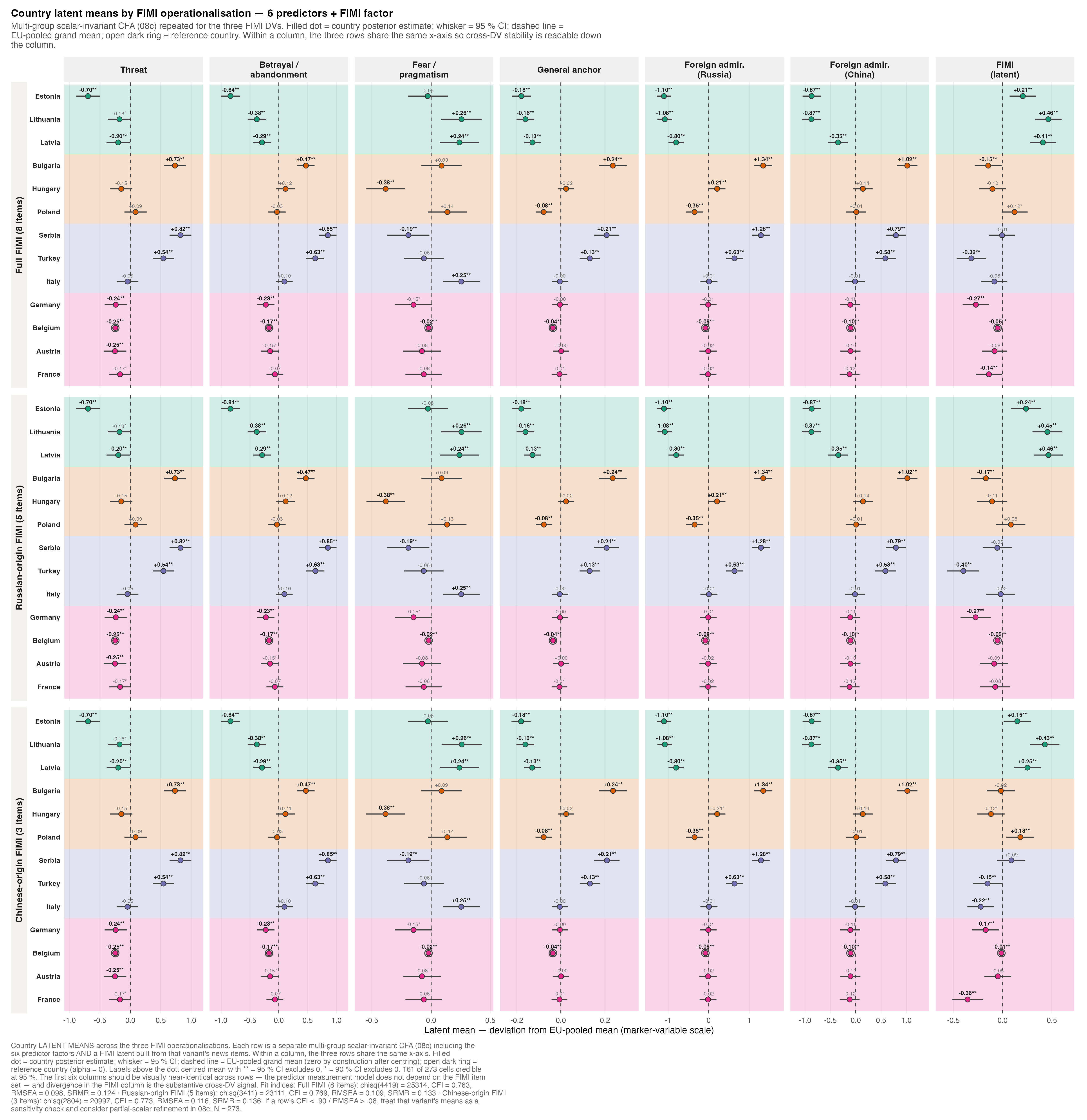
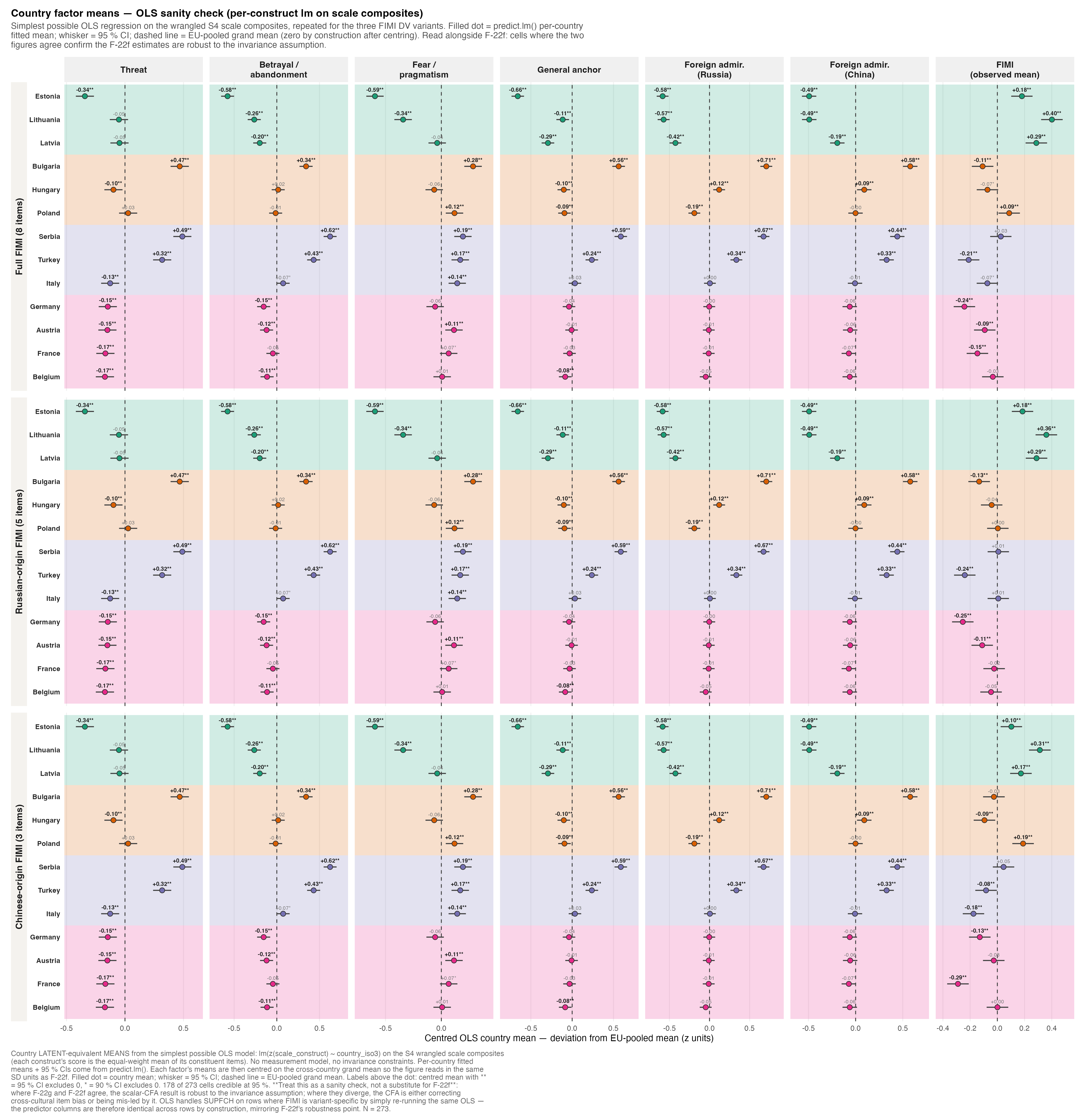
Civic anchors

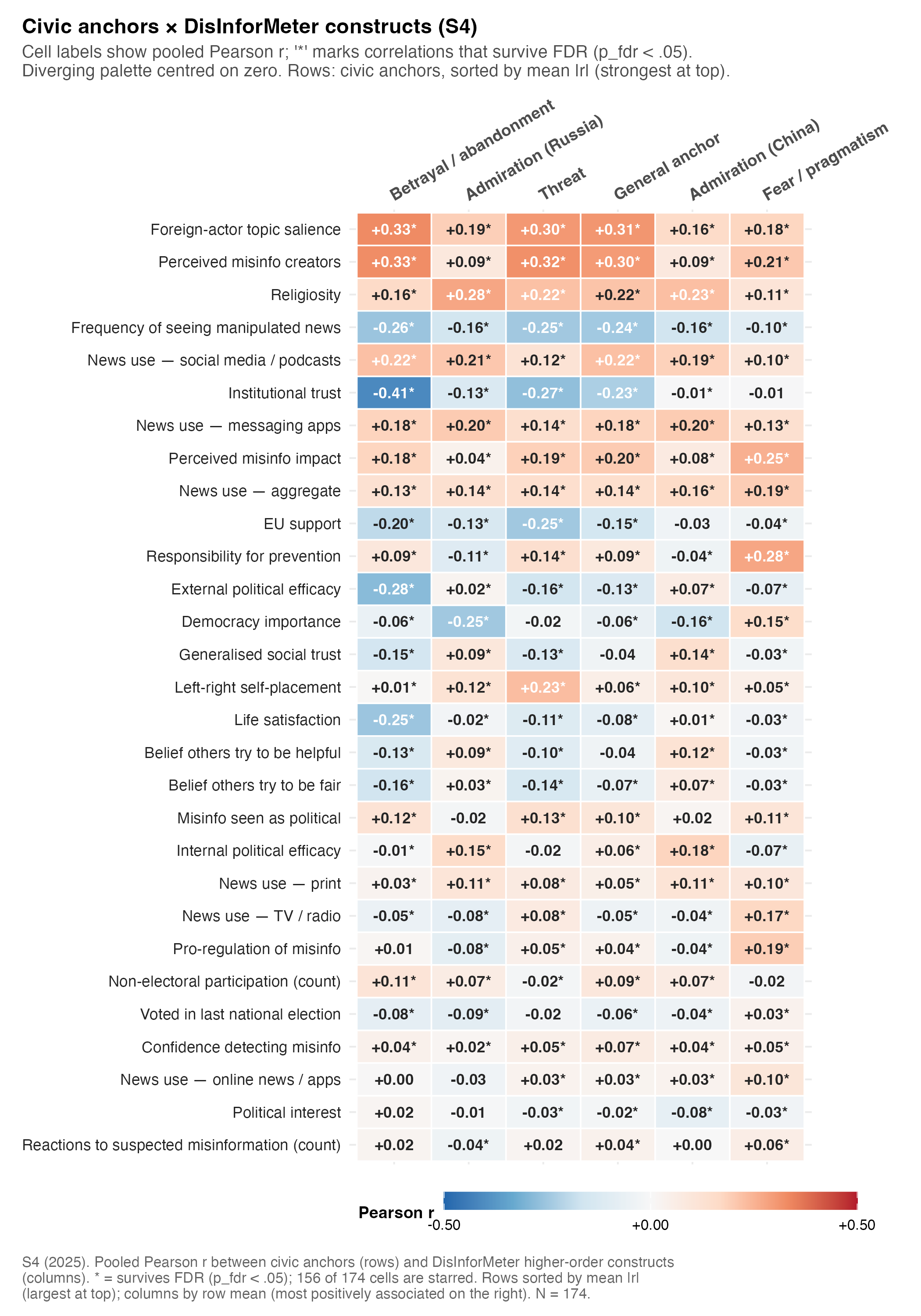
Do the DisInforMeter domains connect to the wider civic conditions that make FIMI resilience stronger or weaker? Betrayal / Abandonment is the clearest institutional-trust construct: it tracks lower institutional trust, external political efficacy, EU support, social trust, and life satisfaction, and higher perceived foreign-actor salience. Threat also tracks lower institutional trust and EU support, while Fear / Pragmatism is tied to perceived misinformation impact and responsibility for prevention (Akkerman et al., 2014; ESS, 2024; Niemi et al., 1991; OECD, 2017).

Figure 8: Civic-anchor correlation heatmap: rows = civic / misinformation anchors, columns = DisInforMeter domains. Cells are pooled Pearson correlations; stars indicate FDR-adjusted significance.

scripts/policy_report/F-20_civic_anchor_heatmap.R

#!/usr/bin/env Rscript
#' F-20 — Civic anchor correlation heatmap (nomological network).
#'
#' Spec: rows = DisInforMeter higher-order construct, columns = civic
#' anchor variable, cell = pooled r. Asterisks mark cells where FDR-
#' corrected p < .05. Divergent palette centred on zero. Rows sorted by
#' row mean.
#'
#' Source CSV: outputs/policy_report/tables/s4_anchor_correlations_wide.csv
#'             outputs/policy_report/tables/s4_anchor_correlations_wide_sig.csv
#'             (twin "*" marker matrix; cells with `*` survive FDR)
#' Output:     outputs/policy_report/figures/F-20_civic_anchor_heatmap.{png,pdf,rds}

suppressPackageStartupMessages({
  library(ggplot2)
  library(dplyr)
  library(tidyr)
  library(readr)
  library(forcats)
  library(here)
})

source(here::here("scripts", "policy_report", "_theme.R"))

SCRIPT_ID  <- "F-20_civic_anchor_heatmap"
SOURCE_CSV <- here::here("outputs", "policy_report", "tables",
                          "s4_anchor_correlations_wide.csv")
SIG_CSV    <- here::here("outputs", "policy_report", "tables",
                          "s4_anchor_correlations_wide_sig.csv")
OUT_BASE   <- file.path(POLICY_REPORT_FIG_DIR, SCRIPT_ID)

set.seed(42)

dat_w <- readr::read_csv(SOURCE_CSV, show_col_types = FALSE)
policy_report_check_input(dat_w, SOURCE_CSV)

sig_w <- readr::read_csv(SIG_CSV, show_col_types = FALSE,
                          col_types = readr::cols(.default = "c"))
policy_report_check_input(sig_w, SIG_CSV)

PREDICTOR_LBL <- c(
  THREAT = "Threat",
  ABAND  = "Betrayal / abandonment",
  FEAR   = "Fear / pragmatism",
  GEN    = "General anchor",
  SUPF   = "Admiration (Russia)",
  SUPFCH = "Admiration (China)"
)

# Pivot correlations to long.
long_r <- dat_w %>%
  tidyr::pivot_longer(-predictor_label,
                      names_to  = "anchor",
                      values_to = "r")

# Pivot significance marks to long; "*" means survived FDR (p_fdr < .05).
long_s <- sig_w %>%
  tidyr::pivot_longer(-predictor_label,
                      names_to  = "anchor",
                      values_to = "sig_mark") %>%
  dplyr::mutate(sig_mark = dplyr::coalesce(sig_mark, ""),
                survived_fdr = sig_mark == "*")

long <- long_r %>%
  dplyr::left_join(long_s, by = c("predictor_label", "anchor")) %>%
  dplyr::mutate(
    construct_lbl = factor(PREDICTOR_LBL[predictor_label],
                            levels = PREDICTOR_LBL),
    cell_label = ifelse(is.na(r), "",
                         sprintf("%+.2f%s", r,
                                  ifelse(survived_fdr, "*", "")))
  )

# Transpose layout: anchors on Y (the longer list, 29 entries), constructs
# on X (6 entries). Cells become tall + narrow but every row label fits
# without rotation. Anchors are sorted top-to-bottom by mean |r| (largest
# correlation block at top); constructs are sorted left-to-right by row
# mean r (most strongly-positive on the right).
anchor_strength <- long %>%
  dplyr::group_by(anchor) %>%
  dplyr::summarise(strength = mean(abs(r), na.rm = TRUE), .groups = "drop") %>%
  dplyr::arrange(strength)        # ascending so largest ends up at top
long <- long %>%
  dplyr::mutate(anchor = factor(anchor, levels = anchor_strength$anchor))

construct_order <- long %>%
  dplyr::group_by(construct_lbl) %>%
  dplyr::summarise(row_mean = mean(r, na.rm = TRUE), .groups = "drop") %>%
  dplyr::arrange(row_mean) %>%
  dplyr::pull(construct_lbl)
long <- long %>%
  dplyr::mutate(construct_lbl = factor(construct_lbl,
                                         levels = construct_order))

# Diverging palette centred on zero. Use a symmetric span derived from the
# data so the gradient never compresses against the extremes.
max_abs <- max(abs(long$r), na.rm = TRUE)
limit_v <- max(0.10, ceiling(max_abs * 10) / 10)

n_sig <- sum(long$survived_fdr, na.rm = TRUE)
n_cells <- nrow(long)

caption <- policy_report_caption(
  source = "outputs/policy_report/tables/s4_anchor_correlations_wide.csv",
  n      = n_cells,
  script = paste0(SCRIPT_ID, ".R"),
  prefix = sprintf("S4 (2025). Pooled Pearson r between civic anchors (rows) and DisInforMeter higher-order constructs (columns). * = survives FDR (p_fdr < .05); %d of %d cells are starred. Rows sorted by mean |r| (largest at top); columns by row mean (most positively associated on the right).",
                   n_sig, n_cells))

p <- ggplot2::ggplot(long,
                     ggplot2::aes(x = construct_lbl, y = anchor,
                                  fill = r)) +
  ggplot2::geom_tile(colour = "white", linewidth = 0.4) +
  ggplot2::geom_text(
    ggplot2::aes(label = cell_label,
                 colour = ifelse(abs(r) > 0.22, "white", "grey15")),
    size = 3.0, fontface = "bold",
    family = .policy_report_resolve_font(POLICY_REPORT_BASE_FONT)
  ) +
  ggplot2::scale_fill_gradientn(
    colours = policy_report_palette("diverging"),
    limits  = c(-limit_v, limit_v),
    breaks  = c(-limit_v, 0, limit_v),
    labels  = sprintf("%+.2f", c(-limit_v, 0, limit_v)),
    oob     = scales::squish,
    name    = "Pearson r"
  ) +
  ggplot2::scale_colour_identity() +
  ggplot2::scale_x_discrete(position = "top") +
  ggplot2::labs(
    title    = "Civic anchors × DisInforMeter constructs (S4)",
    subtitle = policy_report_wrap("Cell labels show pooled Pearson r; '*' marks correlations that survive FDR (p_fdr < .05). Diverging palette centred on zero. Rows: civic anchors, sorted by mean |r| (strongest at top).", width = 95),
    x = NULL, y = NULL,
    caption = caption
  ) +
  # F-20 has very long y-tick labels (civic anchors) that push the panel
  # rightward; bump the right margin via the central `right_extra` mechanism
  # so the diagonal top-axis labels can flow into the extra space instead of
  # being clipped at the canvas edge.
  theme_policy_report(base_size = 10, right_extra = 46) +
  ggplot2::theme(
    panel.grid       = ggplot2::element_blank(),
    axis.ticks       = ggplot2::element_blank(),
    axis.text.x.top  = ggplot2::element_text(angle = 30, hjust = 0,
                                              vjust = 0, size = 9,
                                              face = "bold",
                                              lineheight = 0.9),
    axis.text.x      = ggplot2::element_text(angle = 30, hjust = 0,
                                              vjust = 0, size = 9,
                                              face = "bold",
                                              lineheight = 0.9),
    axis.text.y      = ggplot2::element_text(size = 8.5, colour = "grey15",
                                              hjust = 1),
    legend.position      = "bottom",
    legend.justification = "left",
    legend.box.just      = "left",
    legend.box.margin    = ggplot2::margin(l = 0),
    legend.key.width     = grid::unit(1.6, "cm"),
    legend.key.height    = grid::unit(0.35, "cm")
  )

dim_p <- POLICY_REPORT_FIGURE_DIMENSIONS$full_page
paths <- safe_ggsave_rds(p, OUT_BASE,
                         width  = dim_p$width,
                         height = dim_p$height + 0.5)

policy_report_log_outputs(
  SCRIPT_ID, paths, input_rows = nrow(long),
  extra = c(sprintf("Constructs: %d, Anchors: %d",
                    dplyr::n_distinct(long$construct_lbl),
                    dplyr::n_distinct(long$anchor)),
            sprintf("Cells significant after FDR: %d / %d", n_sig, n_cells),
            sprintf("r range: [%+.2f, %+.2f]",
                    min(long$r, na.rm = TRUE),
                    max(long$r, na.rm = TRUE)),
            sprintf("Palette limit (symmetric): ±%.2f", limit_v)))

Full external-anchor correlations (Annex E.2 — all 174 rows):

Table 2

Annex E.2 — Full external anchor correlations
Pearson correlations between DisInforMeter constructs and external civic anchors (Eurobarometer-style indicators). Significance asterisks reflect the FDR-adjusted p (Benjamini–Hochberg): * p < .05, ** p < .01, *** p < .001.
Predictor	Anchor	Family	N	r (pooled)	p (FDR)
ABAND	Institutional trust	Civic / political	8,040	−0.410	0.0000	***
ABAND	External political efficacy	Civic / political	8,040	−0.283	0.0000	***
ABAND	Life satisfaction	Civic / political	8,040	−0.253	0.0000	***
ABAND	EU support	Civic / political	8,040	−0.197	0.0000	***
ABAND	Religiosity	Civic / political	8,040	0.164	0.0000	***
ABAND	Generalised social trust	Civic / political	8,040	−0.153	0.0000	***
ABAND	Democracy importance	Civic / political	8,040	−0.059	0.0000	***
ABAND	Political interest	Civic / political	8,040	0.017	0.7077
ABAND	Internal political efficacy	Civic / political	8,040	−0.008	0.0108	*
ABAND	Left-right self-placement	Civic / political	8,040	0.007	0.0013	**
FEAR	Democracy importance	Civic / political	8,040	0.151	0.0000	***
FEAR	Religiosity	Civic / political	8,040	0.111	0.0000	***
FEAR	External political efficacy	Civic / political	8,040	−0.071	0.0000	***
FEAR	Internal political efficacy	Civic / political	8,040	−0.067	0.0000	***
FEAR	Left-right self-placement	Civic / political	8,040	0.054	0.0000	***
FEAR	EU support	Civic / political	8,040	−0.039	0.0010	**
FEAR	Life satisfaction	Civic / political	8,040	−0.033	0.0009	***
FEAR	Political interest	Civic / political	8,040	−0.033	0.0020	**
FEAR	Generalised social trust	Civic / political	8,040	−0.030	0.0158	*
FEAR	Institutional trust	Civic / political	8,040	−0.005	0.8823
GEN	Institutional trust	Civic / political	8,040	−0.228	0.0000	***
GEN	Religiosity	Civic / political	8,040	0.215	0.0000	***
GEN	EU support	Civic / political	8,040	−0.152	0.0000	***
GEN	External political efficacy	Civic / political	8,040	−0.125	0.0000	***
GEN	Life satisfaction	Civic / political	8,040	−0.083	0.0000	***
GEN	Democracy importance	Civic / political	8,040	−0.062	0.0000	***
GEN	Internal political efficacy	Civic / political	8,040	0.058	0.0001	***
GEN	Left-right self-placement	Civic / political	8,040	0.056	0.0000	***
GEN	Generalised social trust	Civic / political	8,040	−0.036	0.8853
GEN	Political interest	Civic / political	8,040	−0.018	0.0089	**
SUPF	Religiosity	Civic / political	8,040	0.276	0.0000	***
SUPF	Democracy importance	Civic / political	8,040	−0.246	0.0000	***
SUPF	Internal political efficacy	Civic / political	8,040	0.155	0.0000	***
SUPF	EU support	Civic / political	8,040	−0.135	0.0000	***
SUPF	Institutional trust	Civic / political	8,040	−0.126	0.0026	**
SUPF	Left-right self-placement	Civic / political	8,040	0.122	0.0000	***
SUPF	Generalised social trust	Civic / political	8,040	0.095	0.0000	***
SUPF	Life satisfaction	Civic / political	8,040	−0.023	0.0003	***
SUPF	External political efficacy	Civic / political	8,040	0.023	0.0000	***
SUPF	Political interest	Civic / political	8,040	−0.007	0.1045
SUPFCH	Religiosity	Civic / political	8,040	0.225	0.0000	***
SUPFCH	Internal political efficacy	Civic / political	8,040	0.179	0.0000	***
SUPFCH	Democracy importance	Civic / political	8,040	−0.165	0.0000	***
SUPFCH	Generalised social trust	Civic / political	8,040	0.141	0.0000	***
SUPFCH	Left-right self-placement	Civic / political	8,040	0.101	0.0000	***
SUPFCH	Political interest	Civic / political	8,040	−0.075	0.0000	***
SUPFCH	External political efficacy	Civic / political	8,040	0.070	0.0000	***
SUPFCH	EU support	Civic / political	8,040	−0.034	0.1677
SUPFCH	Life satisfaction	Civic / political	8,040	0.013	0.0000	***
SUPFCH	Institutional trust	Civic / political	8,040	−0.006	0.0000	***
THREAT	Institutional trust	Civic / political	8,040	−0.272	0.0000	***
THREAT	EU support	Civic / political	8,040	−0.247	0.0000	***
THREAT	Left-right self-placement	Civic / political	8,040	0.229	0.0000	***
THREAT	Religiosity	Civic / political	8,040	0.221	0.0000	***
THREAT	External political efficacy	Civic / political	8,040	−0.156	0.0000	***
THREAT	Generalised social trust	Civic / political	8,040	−0.127	0.0000	***
THREAT	Life satisfaction	Civic / political	8,040	−0.115	0.0000	***
THREAT	Political interest	Civic / political	8,040	−0.031	0.0001	***
THREAT	Democracy importance	Civic / political	8,040	−0.020	0.0676
THREAT	Internal political efficacy	Civic / political	8,040	−0.018	0.0895
ABAND	Foreign-actor topic salience	Misinformation	8,040	0.330	0.0000	***
ABAND	Perceived misinfo creators	Misinformation	8,040	0.327	0.0000	***
ABAND	Perceived misinfo impact	Misinformation	8,040	0.177	0.0000	***
ABAND	Misinfo seen as political	Misinformation	8,040	0.116	0.0000	***
ABAND	Responsibility for prevention	Misinformation	8,040	0.094	0.0000	***
ABAND	Confidence detecting misinfo	Misinformation	8,040	0.042	0.0003	***
ABAND	Pro-regulation of misinfo	Misinformation	8,040	0.013	0.5842
FEAR	Responsibility for prevention	Misinformation	8,040	0.276	0.0000	***
FEAR	Perceived misinfo impact	Misinformation	8,040	0.255	0.0000	***
FEAR	Perceived misinfo creators	Misinformation	8,040	0.206	0.0000	***
FEAR	Pro-regulation of misinfo	Misinformation	8,040	0.194	0.0000	***
FEAR	Foreign-actor topic salience	Misinformation	8,040	0.176	0.0000	***
FEAR	Misinfo seen as political	Misinformation	8,040	0.106	0.0000	***
FEAR	Confidence detecting misinfo	Misinformation	8,040	0.045	0.0002	***
GEN	Foreign-actor topic salience	Misinformation	8,040	0.309	0.0000	***
GEN	Perceived misinfo creators	Misinformation	8,040	0.299	0.0000	***
GEN	Perceived misinfo impact	Misinformation	8,040	0.201	0.0000	***
GEN	Misinfo seen as political	Misinformation	8,040	0.103	0.0000	***
GEN	Responsibility for prevention	Misinformation	8,040	0.085	0.0000	***
GEN	Confidence detecting misinfo	Misinformation	8,040	0.074	0.0000	***
GEN	Pro-regulation of misinfo	Misinformation	8,040	0.036	0.0034	**
SUPF	Foreign-actor topic salience	Misinformation	8,040	0.191	0.0000	***
SUPF	Responsibility for prevention	Misinformation	8,040	−0.107	0.0000	***
SUPF	Perceived misinfo creators	Misinformation	8,040	0.090	0.0000	***
SUPF	Pro-regulation of misinfo	Misinformation	8,040	−0.084	0.0000	***
SUPF	Perceived misinfo impact	Misinformation	8,040	0.037	0.0000	***
SUPF	Misinfo seen as political	Misinformation	8,040	−0.019	0.0616
SUPF	Confidence detecting misinfo	Misinformation	8,040	0.017	0.0302	*
SUPFCH	Foreign-actor topic salience	Misinformation	8,040	0.159	0.0000	***
SUPFCH	Perceived misinfo creators	Misinformation	8,040	0.088	0.0000	***
SUPFCH	Perceived misinfo impact	Misinformation	8,040	0.077	0.0000	***
SUPFCH	Confidence detecting misinfo	Misinformation	8,040	0.043	0.0000	***
SUPFCH	Responsibility for prevention	Misinformation	8,040	−0.040	0.0010	***
SUPFCH	Pro-regulation of misinfo	Misinformation	8,040	−0.040	0.0001	***
SUPFCH	Misinfo seen as political	Misinformation	8,040	0.016	0.1649
THREAT	Perceived misinfo creators	Misinformation	8,040	0.321	0.0000	***
THREAT	Foreign-actor topic salience	Misinformation	8,040	0.304	0.0000	***
THREAT	Perceived misinfo impact	Misinformation	8,040	0.187	0.0000	***
THREAT	Responsibility for prevention	Misinformation	8,040	0.140	0.0000	***
THREAT	Misinfo seen as political	Misinformation	8,040	0.134	0.0000	***
THREAT	Confidence detecting misinfo	Misinformation	8,040	0.047	0.0002	***
THREAT	Pro-regulation of misinfo	Misinformation	8,040	0.045	0.0001	***
ABAND	Frequency of seeing manipulated news	Prereg #8 behavioural / participation	8,040	−0.256	0.0000	***
ABAND	Non-electoral participation (count)	Prereg #8 behavioural / participation	8,040	0.112	0.0000	***
ABAND	Voted in last national election	Prereg #8 behavioural / participation	7,912	−0.080	0.0000	***
ABAND	Reactions to suspected misinformation (count)	Prereg #8 behavioural / participation	8,040	0.023	0.2989
FEAR	Frequency of seeing manipulated news	Prereg #8 behavioural / participation	8,040	−0.104	0.0000	***
FEAR	Reactions to suspected misinformation (count)	Prereg #8 behavioural / participation	8,040	0.058	0.0000	***
FEAR	Voted in last national election	Prereg #8 behavioural / participation	7,912	0.034	0.0024	**
FEAR	Non-electoral participation (count)	Prereg #8 behavioural / participation	8,040	−0.023	0.0820
GEN	Frequency of seeing manipulated news	Prereg #8 behavioural / participation	8,040	−0.245	0.0000	***
GEN	Non-electoral participation (count)	Prereg #8 behavioural / participation	8,040	0.094	0.0000	***
GEN	Voted in last national election	Prereg #8 behavioural / participation	7,912	−0.056	0.0004	***
GEN	Reactions to suspected misinformation (count)	Prereg #8 behavioural / participation	8,040	0.036	0.0019	**
SUPF	Frequency of seeing manipulated news	Prereg #8 behavioural / participation	8,040	−0.159	0.0000	***
SUPF	Voted in last national election	Prereg #8 behavioural / participation	7,912	−0.088	0.0000	***
SUPF	Non-electoral participation (count)	Prereg #8 behavioural / participation	8,040	0.066	0.0002	***
SUPF	Reactions to suspected misinformation (count)	Prereg #8 behavioural / participation	8,040	−0.040	0.0007	***
SUPFCH	Frequency of seeing manipulated news	Prereg #8 behavioural / participation	8,040	−0.164	0.0000	***
SUPFCH	Non-electoral participation (count)	Prereg #8 behavioural / participation	8,040	0.068	0.0000	***
SUPFCH	Voted in last national election	Prereg #8 behavioural / participation	7,912	−0.045	0.0435	*
SUPFCH	Reactions to suspected misinformation (count)	Prereg #8 behavioural / participation	8,040	0.001	0.9165
THREAT	Frequency of seeing manipulated news	Prereg #8 behavioural / participation	8,040	−0.245	0.0000	***
THREAT	Voted in last national election	Prereg #8 behavioural / participation	7,912	−0.024	0.0759
THREAT	Reactions to suspected misinformation (count)	Prereg #8 behavioural / participation	8,040	0.022	0.6356
THREAT	Non-electoral participation (count)	Prereg #8 behavioural / participation	8,040	−0.019	0.0045	**
ABAND	Belief others try to be fair	Prereg #8 convergent fairness / helpfulness	8,040	−0.164	0.0000	***
ABAND	Belief others try to be helpful	Prereg #8 convergent fairness / helpfulness	8,040	−0.132	0.0000	***
FEAR	Belief others try to be fair	Prereg #8 convergent fairness / helpfulness	8,040	−0.034	0.0105	*
FEAR	Belief others try to be helpful	Prereg #8 convergent fairness / helpfulness	8,040	−0.031	0.0183	*
GEN	Belief others try to be fair	Prereg #8 convergent fairness / helpfulness	8,040	−0.069	0.0106	*
GEN	Belief others try to be helpful	Prereg #8 convergent fairness / helpfulness	8,040	−0.036	0.5716
SUPF	Belief others try to be helpful	Prereg #8 convergent fairness / helpfulness	8,040	0.085	0.0000	***
SUPF	Belief others try to be fair	Prereg #8 convergent fairness / helpfulness	8,040	0.026	0.0000	***
SUPFCH	Belief others try to be helpful	Prereg #8 convergent fairness / helpfulness	8,040	0.120	0.0000	***
SUPFCH	Belief others try to be fair	Prereg #8 convergent fairness / helpfulness	8,040	0.069	0.0000	***
THREAT	Belief others try to be fair	Prereg #8 convergent fairness / helpfulness	8,040	−0.140	0.0000	***
THREAT	Belief others try to be helpful	Prereg #8 convergent fairness / helpfulness	8,040	−0.100	0.0000	***
ABAND	News use — social media / podcasts	Prereg #8 media-channel use	8,040	0.222	0.0000	***
ABAND	News use — messaging apps	Prereg #8 media-channel use	8,040	0.181	0.0000	***
ABAND	News use — aggregate	Prereg #8 media-channel use	8,040	0.129	0.0000	***
ABAND	News use — TV / radio	Prereg #8 media-channel use	8,040	−0.053	0.0000	***
ABAND	News use — print	Prereg #8 media-channel use	8,040	0.028	0.0075	**
ABAND	News use — online news / apps	Prereg #8 media-channel use	8,040	0.004	0.6165
FEAR	News use — aggregate	Prereg #8 media-channel use	8,040	0.195	0.0000	***
FEAR	News use — TV / radio	Prereg #8 media-channel use	8,040	0.171	0.0000	***
FEAR	News use — messaging apps	Prereg #8 media-channel use	8,040	0.134	0.0000	***
FEAR	News use — social media / podcasts	Prereg #8 media-channel use	8,040	0.105	0.0000	***
FEAR	News use — online news / apps	Prereg #8 media-channel use	8,040	0.102	0.0000	***
FEAR	News use — print	Prereg #8 media-channel use	8,040	0.098	0.0000	***
GEN	News use — social media / podcasts	Prereg #8 media-channel use	8,040	0.222	0.0000	***
GEN	News use — messaging apps	Prereg #8 media-channel use	8,040	0.179	0.0000	***
GEN	News use — aggregate	Prereg #8 media-channel use	8,040	0.145	0.0000	***
GEN	News use — print	Prereg #8 media-channel use	8,040	0.050	0.0000	***
GEN	News use — TV / radio	Prereg #8 media-channel use	8,040	−0.045	0.0000	***
GEN	News use — online news / apps	Prereg #8 media-channel use	8,040	0.026	0.0008	***
SUPF	News use — social media / podcasts	Prereg #8 media-channel use	8,040	0.207	0.0000	***
SUPF	News use — messaging apps	Prereg #8 media-channel use	8,040	0.201	0.0000	***
SUPF	News use — aggregate	Prereg #8 media-channel use	8,040	0.135	0.0000	***
SUPF	News use — print	Prereg #8 media-channel use	8,040	0.108	0.0000	***
SUPF	News use — TV / radio	Prereg #8 media-channel use	8,040	−0.081	0.0000	***
SUPF	News use — online news / apps	Prereg #8 media-channel use	8,040	−0.035	0.0738
SUPFCH	News use — messaging apps	Prereg #8 media-channel use	8,040	0.198	0.0000	***
SUPFCH	News use — social media / podcasts	Prereg #8 media-channel use	8,040	0.185	0.0000	***
SUPFCH	News use — aggregate	Prereg #8 media-channel use	8,040	0.163	0.0000	***
SUPFCH	News use — print	Prereg #8 media-channel use	8,040	0.113	0.0000	***
SUPFCH	News use — TV / radio	Prereg #8 media-channel use	8,040	−0.036	0.0007	***
SUPFCH	News use — online news / apps	Prereg #8 media-channel use	8,040	0.033	0.0000	***
THREAT	News use — aggregate	Prereg #8 media-channel use	8,040	0.144	0.0000	***
THREAT	News use — messaging apps	Prereg #8 media-channel use	8,040	0.141	0.0000	***
THREAT	News use — social media / podcasts	Prereg #8 media-channel use	8,040	0.118	0.0000	***
THREAT	News use — TV / radio	Prereg #8 media-channel use	8,040	0.076	0.0000	***
THREAT	News use — print	Prereg #8 media-channel use	8,040	0.076	0.0000	***
THREAT	News use — online news / apps	Prereg #8 media-channel use	8,040	0.030	0.0086	**
Source: outputs/tables/s4_external_anchor_correlations.csv (pooled r, FDR-adjusted p, ranked by |r|). N = 8,040. Reproduction code: scripts/policy_report/A-07_anchor_correlations.R.

External validation (Study 5)

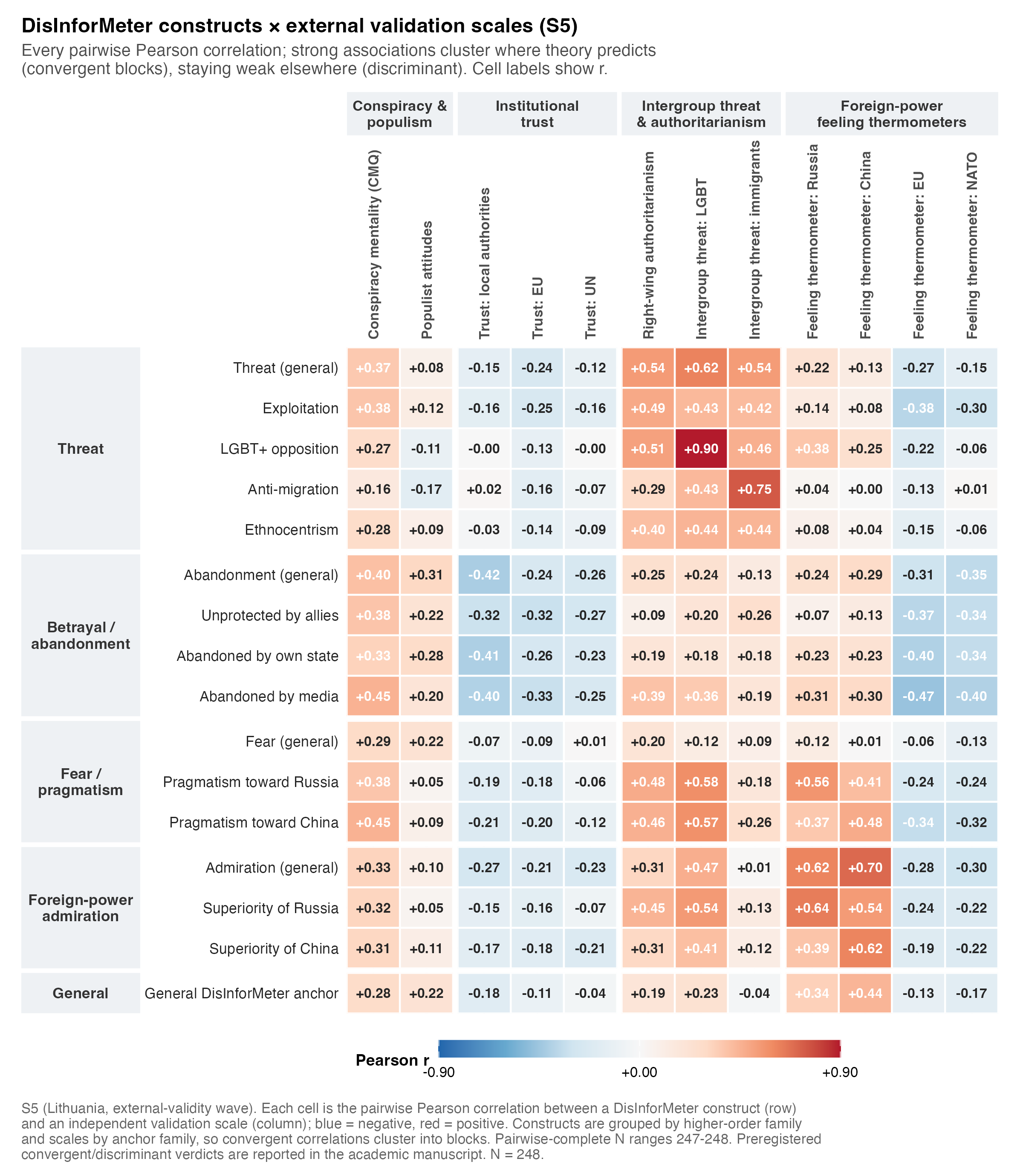
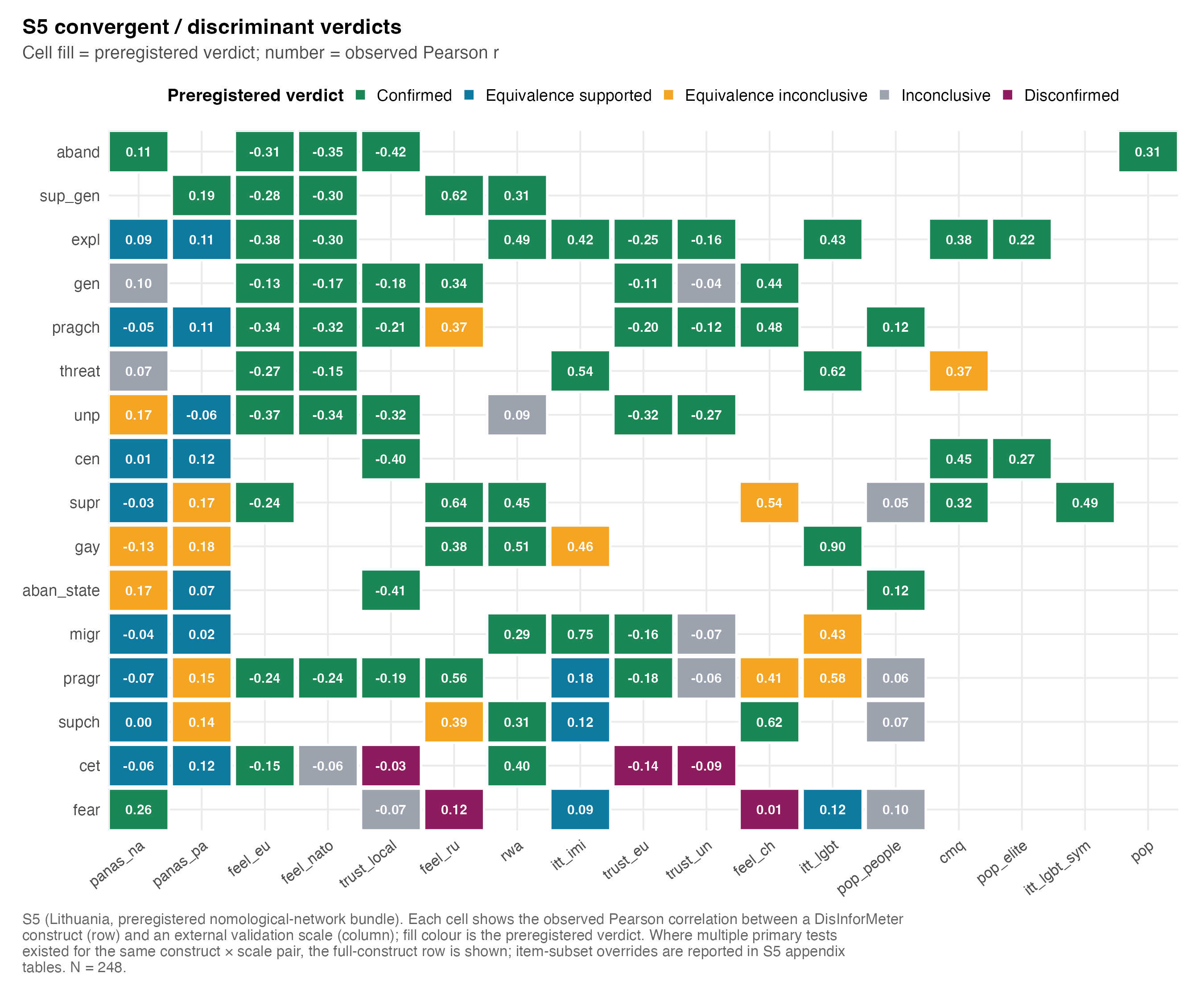
Study 5 correlated every DisInforMeter construct against a battery of established scales. Three patterns stand out, and together they place the domains cleanly in the wider nomological network (Bruder et al., 2013; Campbell & Fiske, 1959; Stephan et al., 2009):

1. Convergence is exactly where theory predicts. Opposition to LGBT+ rights tracks the matching intergroup-threat scale almost one-to-one ((r = .90)); anti-migration tracks immigrant intergroup threat ((r = .75)); foreign-power admiration tracks warmth toward Russia and China ((r )–(.7)), and with the correct target (Russia items ↔︎ Russia thermometer, China items ↔︎ China thermometer).
2. The construct families separate cleanly. Betrayal/Abandonment is the institutional-distrust/populism construct (≈ (-.4) with institutional trust), whereas the threat constructs are largely unrelated to trust — a double dissociation no undifferentiated negativity factor could produce.
3. It is neither a conspiracy scale nor a negativity halo. Associations with generic conspiracy mentality are only moderate and uniform (≈ (.3)); admiration raises warmth toward Russia/China while lowering it toward the EU and NATO.

Figure 9: S5 external-validation correlation matrix. Each cell is the pairwise Pearson correlation between a DisInforMeter construct (row) and an independent validation scale (column); blue = negative, red = positive. Convergent associations form visible blocks; discriminant pairs stay pale.

Figure 10: S5 preregistered-hypothesis verdict panel: which preregistered convergent/discriminant predictions were supported.

S5 preregistered-hypothesis verdicts (Annex E.3):

Table 3

Annex E.3 — S5 preregistered hypothesis verdicts
Each row is a preregistered convergent / discriminant test between a DisInforMeter construct and an external validation instrument. Verdicts are computed from observed r, the two one-sided tests (TOST) for equivalence, and the preregistered region of practical equivalence.
Construct	Validation instrument	Hypothesised sign	N	r	95 % CI	p (two-sided)	Verdict
Abandoned [general]	Institutional trust battery (ESS) - Local Authorities	-	248	-0.42	[-0.52, -0.31]	0.0000	confirmed
Abandoned [general]	Institutional trust battery (ESS) - Local Authorities	-	248	-0.42	[-0.52, -0.31]	0.0000	confirmed
Abandoned [general]	Populist attitudes scale (Silva, 2017)	+	248	0.31	[0.19, 0.42]	0.0000	confirmed
Abandoned [general]	Populist attitudes scale (Silva, 2017)	+	248	0.29	[0.17, 0.40]	0.0000	confirmed
Abandoned [general]	Trait affectivity (I‑PANAS‑SF)	+	247	0.11	[-0.01, 0.24]	0.0723	confirmed
Abandoned [general]	feeling thermometer - EU	-	248	-0.31	[-0.42, -0.19]	0.0000	confirmed
Abandoned [general]	feeling thermometer - NATO	-	248	-0.35	[-0.46, -0.24]	0.0000	confirmed
Abandoned by media (censorship)	Conspiracy Mentality Questionnaire (CMQ; 5-item)	+	248	0.45	[0.35, 0.55]	0.0000	confirmed
Abandoned by media (censorship)	Institutional trust battery (ESS) - Local Authorities	-	248	-0.40	[-0.50, -0.28]	0.0000	confirmed
Abandoned by media (censorship)	Populist attitudes scale (Silva, 2017)	+	248	0.27	[0.15, 0.38]	0.0000	confirmed
Abandoned by media (censorship)	Populist attitudes scale (Silva, 2017)	+	248	0.21	[0.09, 0.33]	0.0007	confirmed
Abandoned by media (censorship)	Trait affectivity (I‑PANAS‑SF)	0	248	0.12	[-0.00, 0.25]	0.0501	equivalence_supported
Abandoned by media (censorship)	Trait affectivity (I‑PANAS‑SF)	0	247	0.01	[-0.11, 0.14]	0.8495	equivalence_supported
Abandoned by own state	Institutional trust battery (ESS) - Local Authorities	-	248	-0.41	[-0.51, -0.30]	0.0000	confirmed
Abandoned by own state	Populist attitudes scale (Silva, 2017)	+	248	0.12	[-0.01, 0.24]	0.0612	confirmed
Abandoned by own state	Trait affectivity (I‑PANAS‑SF)	0	248	0.07	[-0.06, 0.19]	0.2880	equivalence_supported
Abandoned by own state	Trait affectivity (I‑PANAS‑SF)	0	247	0.17	[0.05, 0.29]	0.0060	equivalence_inconclusive
Exploitation	Conspiracy Mentality Questionnaire (CMQ; 5-item)	+	248	0.38	[0.27, 0.48]	0.0000	confirmed
Exploitation	Institutional trust battery (ESS) - EU	-	248	-0.25	[-0.36, -0.12]	0.0001	confirmed
Exploitation	Institutional trust battery (ESS) - United Nations	-	248	-0.16	[-0.28, -0.04]	0.0096	confirmed
Exploitation	Intergroup threat scale (ITT) - Immigrants	+	248	0.42	[0.31, 0.52]	0.0000	confirmed
Exploitation	Intergroup threat scale (ITT) - Immigrants	+	248	0.41	[0.30, 0.51]	0.0000	confirmed
Exploitation	Intergroup threat scale (ITT) - LQBT	+	248	0.43	[0.32, 0.52]	0.0000	confirmed
Exploitation	Intergroup threat scale (ITT) - LQBT	+	248	0.29	[0.17, 0.40]	0.0000	confirmed
Exploitation	Populist attitudes scale (Silva, 2017)	+	248	0.22	[0.10, 0.33]	0.0006	confirmed
Exploitation	Right Wing Authoritarianism (RWA short scale)	+	248	0.49	[0.39, 0.58]	0.0000	confirmed
Exploitation	Trait affectivity (I‑PANAS‑SF)	0	248	0.11	[-0.02, 0.23]	0.0859	equivalence_supported
Exploitation	Trait affectivity (I‑PANAS‑SF)	0	247	0.09	[-0.03, 0.21]	0.1516	equivalence_supported
Exploitation	feeling thermometer - EU	-	248	-0.38	[-0.48, -0.26]	0.0000	confirmed
Exploitation	feeling thermometer - NATO	-	248	-0.30	[-0.41, -0.19]	0.0000	confirmed
Fear [general]	Institutional trust battery (ESS) - Local Authorities	-	248	-0.07	[-0.20, 0.05]	0.2478	inconclusive
Fear [general]	Intergroup threat scale (ITT) - Immigrants	0	248	0.09	[-0.03, 0.21]	0.1482	equivalence_supported
Fear [general]	Intergroup threat scale (ITT) - LQBT	0	248	0.12	[-0.00, 0.24]	0.0548	equivalence_supported
Fear [general]	Populist attitudes scale (Silva, 2017)	+	248	0.10	[-0.02, 0.23]	0.1028	inconclusive
Fear [general]	Trait affectivity (I‑PANAS‑SF)	+	247	0.26	[0.14, 0.37]	0.0000	confirmed
Fear [general]	feeling thermometer - China	u	247	0.01	[-0.12, 0.13]	0.9086	disconfirmed
Fear [general]	feeling thermometer - Russia	u	247	0.12	[-0.00, 0.24]	0.0573	disconfirmed
General	Institutional trust battery (ESS) - EU	-	248	-0.11	[-0.23, 0.02]	0.0964	confirmed
General	Institutional trust battery (ESS) - EU	-	248	-0.11	[-0.23, 0.01]	0.0743	confirmed
General	Institutional trust battery (ESS) - Local Authorities	-	248	-0.18	[-0.30, -0.06]	0.0040	confirmed
General	Institutional trust battery (ESS) - Local Authorities	-	248	-0.16	[-0.28, -0.04]	0.0094	confirmed
General	Institutional trust battery (ESS) - United Nations	-	248	-0.04	[-0.16, 0.09]	0.5398	inconclusive
General	Institutional trust battery (ESS) - United Nations	-	248	-0.13	[-0.25, -0.00]	0.0456	confirmed
General	Trait affectivity (I‑PANAS‑SF)	+	247	0.10	[-0.03, 0.22]	0.1202	inconclusive
General	feeling thermometer - China	+	247	0.44	[0.33, 0.54]	0.0000	confirmed
General	feeling thermometer - China	+	247	0.34	[0.22, 0.44]	0.0000	confirmed
General	feeling thermometer - EU	-	248	-0.13	[-0.25, -0.00]	0.0416	confirmed
General	feeling thermometer - EU	-	248	-0.03	[-0.15, 0.10]	0.6620	inconclusive
General	feeling thermometer - NATO	-	248	-0.17	[-0.29, -0.04]	0.0078	confirmed
General	feeling thermometer - NATO	-	248	-0.12	[-0.24, 0.00]	0.0578	confirmed
General	feeling thermometer - Russia	+	247	0.34	[0.22, 0.44]	0.0000	confirmed
General	feeling thermometer - Russia	+	247	0.61	[0.53, 0.69]	0.0000	confirmed
Immigration	Institutional trust battery (ESS) - EU	-	248	-0.16	[-0.28, -0.04]	0.0092	confirmed
Immigration	Institutional trust battery (ESS) - United Nations	-	248	-0.07	[-0.20, 0.05]	0.2485	inconclusive
Immigration	Intergroup threat scale (ITT) - Immigrants	+	248	0.75	[0.69, 0.80]	0.0000	confirmed
Immigration	Intergroup threat scale (ITT) - LQBT	0	248	0.43	[0.32, 0.53]	0.0000	equivalence_inconclusive
Immigration	Right Wing Authoritarianism (RWA short scale)	+	248	0.29	[0.17, 0.40]	0.0000	confirmed
Immigration	Trait affectivity (I‑PANAS‑SF)	0	248	0.02	[-0.11, 0.14]	0.7717	equivalence_supported
Immigration	Trait affectivity (I‑PANAS‑SF)	0	247	-0.04	[-0.17, 0.08]	0.5126	equivalence_supported
Poisonous ethnocentrism	Institutional trust battery (ESS) - EU	+	248	-0.14	[-0.26, -0.02]	0.0280	disconfirmed
Poisonous ethnocentrism	Institutional trust battery (ESS) - Local Authorities	+	248	-0.03	[-0.15, 0.10]	0.6623	disconfirmed
Poisonous ethnocentrism	Institutional trust battery (ESS) - United Nations	+	248	-0.09	[-0.21, 0.03]	0.1470	disconfirmed
Poisonous ethnocentrism	Right Wing Authoritarianism (RWA short scale)	+	248	0.40	[0.29, 0.50]	0.0000	confirmed
Poisonous ethnocentrism	Trait affectivity (I‑PANAS‑SF)	0	248	0.12	[-0.00, 0.24]	0.0558	equivalence_supported
Poisonous ethnocentrism	Trait affectivity (I‑PANAS‑SF)	0	247	-0.06	[-0.19, 0.06]	0.3153	equivalence_supported
Poisonous ethnocentrism	feeling thermometer - EU	-	248	-0.15	[-0.27, -0.03]	0.0170	confirmed
Poisonous ethnocentrism	feeling thermometer - NATO	-	248	-0.06	[-0.19, 0.06]	0.3150	inconclusive
Pragmatism China	Institutional trust battery (ESS) - EU	-	248	-0.20	[-0.32, -0.08]	0.0017	confirmed
Pragmatism China	Institutional trust battery (ESS) - EU	-	248	-0.10	[-0.22, 0.03]	0.1256	inconclusive
Pragmatism China	Institutional trust battery (ESS) - Local Authorities	-	248	-0.21	[-0.33, -0.09]	0.0007	confirmed
Pragmatism China	Institutional trust battery (ESS) - United Nations	-	248	-0.12	[-0.24, 0.00]	0.0569	confirmed
Pragmatism China	Institutional trust battery (ESS) - United Nations	-	248	-0.02	[-0.14, 0.10]	0.7557	inconclusive
Pragmatism China	Populist attitudes scale (Silva, 2017)	+	248	0.12	[-0.01, 0.24]	0.0619	confirmed
Pragmatism China	Trait affectivity (I‑PANAS‑SF)	0	248	0.11	[-0.02, 0.23]	0.0885	equivalence_supported
Pragmatism China	Trait affectivity (I‑PANAS‑SF)	0	247	-0.05	[-0.17, 0.08]	0.4436	equivalence_supported
Pragmatism China	feeling thermometer - China	+	247	0.48	[0.38, 0.57]	0.0000	confirmed
Pragmatism China	feeling thermometer - China	u	247	0.48	[0.38, 0.57]	0.0000	disconfirmed
Pragmatism China	feeling thermometer - EU	-	248	-0.34	[-0.45, -0.23]	0.0000	confirmed
Pragmatism China	feeling thermometer - EU	-	248	-0.11	[-0.23, 0.01]	0.0810	confirmed
Pragmatism China	feeling thermometer - NATO	-	248	-0.32	[-0.42, -0.20]	0.0000	confirmed
Pragmatism China	feeling thermometer - NATO	-	248	-0.13	[-0.25, -0.01]	0.0411	confirmed
Pragmatism China	feeling thermometer - Russia	0	247	0.37	[0.26, 0.47]	0.0000	equivalence_inconclusive
Pragmatism Russia	Institutional trust battery (ESS) - EU	-	248	-0.18	[-0.30, -0.06]	0.0040	confirmed
Pragmatism Russia	Institutional trust battery (ESS) - EU	-	248	-0.10	[-0.22, 0.03]	0.1256	inconclusive
Pragmatism Russia	Institutional trust battery (ESS) - Local Authorities	-	248	-0.19	[-0.30, -0.06]	0.0034	confirmed
Pragmatism Russia	Institutional trust battery (ESS) - United Nations	-	248	-0.06	[-0.18, 0.07]	0.3659	inconclusive
Pragmatism Russia	Institutional trust battery (ESS) - United Nations	-	248	-0.02	[-0.14, 0.10]	0.7557	inconclusive
Pragmatism Russia	Intergroup threat scale (ITT) - Immigrants	0	248	0.18	[0.05, 0.30]	0.0050	equivalence_supported
Pragmatism Russia	Intergroup threat scale (ITT) - LQBT	0	248	0.58	[0.49, 0.66]	0.0000	equivalence_inconclusive
Pragmatism Russia	Populist attitudes scale (Silva, 2017)	+	248	0.06	[-0.07, 0.18]	0.3573	inconclusive
Pragmatism Russia	Trait affectivity (I‑PANAS‑SF)	0	248	0.15	[0.03, 0.27]	0.0154	equivalence_inconclusive
Pragmatism Russia	Trait affectivity (I‑PANAS‑SF)	0	247	-0.07	[-0.19, 0.06]	0.2996	equivalence_supported
Pragmatism Russia	feeling thermometer - China	0	247	0.41	[0.30, 0.51]	0.0000	equivalence_inconclusive
Pragmatism Russia	feeling thermometer - EU	-	248	-0.24	[-0.35, -0.11]	0.0002	confirmed
Pragmatism Russia	feeling thermometer - EU	-	248	-0.11	[-0.23, 0.01]	0.0810	confirmed
Pragmatism Russia	feeling thermometer - NATO	-	248	-0.24	[-0.36, -0.12]	0.0001	confirmed
Pragmatism Russia	feeling thermometer - NATO	-	248	-0.13	[-0.25, -0.01]	0.0411	confirmed
Pragmatism Russia	feeling thermometer - Russia	+	247	0.56	[0.47, 0.64]	0.0000	confirmed
Pragmatism Russia	feeling thermometer - Russia	u	247	0.56	[0.47, 0.64]	0.0000	confirmed
Queer Sentiment	Intergroup threat scale (ITT) - Immigrants	0	248	0.46	[0.36, 0.56]	0.0000	equivalence_inconclusive
Queer Sentiment	Intergroup threat scale (ITT) - LQBT	+	248	0.90	[0.87, 0.92]	0.0000	confirmed
Queer Sentiment	Right Wing Authoritarianism (RWA short scale)	+	248	0.51	[0.42, 0.60]	0.0000	confirmed
Queer Sentiment	Trait affectivity (I‑PANAS‑SF)	0	248	0.18	[0.06, 0.30]	0.0036	equivalence_inconclusive
Queer Sentiment	Trait affectivity (I‑PANAS‑SF)	0	247	-0.13	[-0.25, -0.01]	0.0386	equivalence_inconclusive
Queer Sentiment	feeling thermometer - Russia	+	247	0.38	[0.27, 0.48]	0.0000	confirmed
Queer Sentiment	feeling thermometer - Russia	+	247	0.42	[0.31, 0.52]	0.0000	confirmed
Superiority China	Intergroup threat scale (ITT) - Immigrants	0	248	0.12	[-0.01, 0.24]	0.0620	equivalence_supported
Superiority China	Populist attitudes scale (Silva, 2017)	+	248	0.07	[-0.06, 0.19]	0.3055	inconclusive
Superiority China	Populist attitudes scale (Silva, 2017)	+	248	0.04	[-0.08, 0.17]	0.5027	inconclusive
Superiority China	Right Wing Authoritarianism (RWA short scale)	+	248	0.31	[0.19, 0.41]	0.0000	confirmed
Superiority China	Trait affectivity (I‑PANAS‑SF)	0	248	0.14	[0.01, 0.26]	0.0302	equivalence_inconclusive
Superiority China	Trait affectivity (I‑PANAS‑SF)	0	247	0.00	[-0.12, 0.13]	0.9447	equivalence_supported
Superiority China	feeling thermometer - China	+	247	0.62	[0.53, 0.69]	0.0000	confirmed
Superiority China	feeling thermometer - Russia	0	247	0.39	[0.27, 0.49]	0.0000	equivalence_inconclusive
Superiority Russia	Conspiracy Mentality Questionnaire (CMQ; 5-item)	+	248	0.32	[0.20, 0.43]	0.0000	confirmed
Superiority Russia	Intergroup threat scale (ITT) - LQBT	+	248	0.49	[0.39, 0.58]	0.0000	confirmed
Superiority Russia	Intergroup threat scale (ITT) - LQBT	+	248	0.46	[0.36, 0.55]	0.0000	confirmed
Superiority Russia	Populist attitudes scale (Silva, 2017)	+	248	0.05	[-0.07, 0.17]	0.4300	inconclusive
Superiority Russia	Right Wing Authoritarianism (RWA short scale)	+	248	0.45	[0.34, 0.54]	0.0000	confirmed
Superiority Russia	Trait affectivity (I‑PANAS‑SF)	0	248	0.17	[0.05, 0.29]	0.0065	equivalence_inconclusive
Superiority Russia	Trait affectivity (I‑PANAS‑SF)	0	247	-0.03	[-0.15, 0.10]	0.6766	equivalence_supported
Superiority Russia	feeling thermometer - China	0	247	0.54	[0.44, 0.62]	0.0000	equivalence_inconclusive
Superiority Russia	feeling thermometer - EU	-	248	-0.24	[-0.36, -0.12]	0.0001	confirmed
Superiority Russia	feeling thermometer - EU	-	248	-0.13	[-0.25, -0.00]	0.0436	confirmed
Superiority Russia	feeling thermometer - Russia	+	247	0.64	[0.56, 0.71]	0.0000	confirmed
Superiority [general]	Right Wing Authoritarianism (RWA short scale)	+	248	0.31	[0.20, 0.42]	0.0000	confirmed
Superiority [general]	Trait affectivity (I‑PANAS‑SF)	+	248	0.19	[0.07, 0.31]	0.0028	confirmed
Superiority [general]	feeling thermometer - EU	-	248	-0.28	[-0.39, -0.16]	0.0000	confirmed
Superiority [general]	feeling thermometer - NATO	-	248	-0.30	[-0.41, -0.18]	0.0000	confirmed
Superiority [general]	feeling thermometer - Russia	+	247	0.62	[0.53, 0.69]	0.0000	confirmed
Threat [general]	Conspiracy Mentality Questionnaire (CMQ; 5-item)	0	248	0.37	[0.25, 0.47]	0.0000	equivalence_inconclusive
Threat [general]	Intergroup threat scale (ITT) - Immigrants	+	248	0.54	[0.44, 0.62]	0.0000	confirmed
Threat [general]	Intergroup threat scale (ITT) - Immigrants	+	248	0.59	[0.50, 0.66]	0.0000	confirmed
Threat [general]	Intergroup threat scale (ITT) - LQBT	+	248	0.62	[0.54, 0.69]	0.0000	confirmed
Threat [general]	Intergroup threat scale (ITT) - LQBT	+	248	0.85	[0.81, 0.88]	0.0000	confirmed
Threat [general]	Trait affectivity (I‑PANAS‑SF)	+	247	0.07	[-0.06, 0.19]	0.2812	inconclusive
Threat [general]	feeling thermometer - EU	-	248	-0.27	[-0.38, -0.15]	0.0000	confirmed
Threat [general]	feeling thermometer - EU	-	248	-0.26	[-0.37, -0.14]	0.0000	confirmed
Threat [general]	feeling thermometer - NATO	-	248	-0.15	[-0.27, -0.03]	0.0186	confirmed
Threat [general]	feeling thermometer - NATO	-	248	-0.28	[-0.39, -0.16]	0.0000	confirmed
Unprotected by international allies	Institutional trust battery (ESS) - EU	-	248	-0.32	[-0.43, -0.20]	0.0000	confirmed
Unprotected by international allies	Institutional trust battery (ESS) - Local Authorities	-	248	-0.32	[-0.42, -0.20]	0.0000	confirmed
Unprotected by international allies	Institutional trust battery (ESS) - United Nations	-	248	-0.27	[-0.39, -0.15]	0.0000	confirmed
Unprotected by international allies	Right Wing Authoritarianism (RWA short scale)	+	248	0.09	[-0.04, 0.21]	0.1716	inconclusive
Unprotected by international allies	Right Wing Authoritarianism (RWA short scale)	+	248	0.10	[-0.02, 0.22]	0.1072	inconclusive
Unprotected by international allies	Trait affectivity (I‑PANAS‑SF)	0	248	-0.06	[-0.18, 0.07]	0.3572	equivalence_supported
Unprotected by international allies	Trait affectivity (I‑PANAS‑SF)	0	247	0.17	[0.05, 0.29]	0.0077	equivalence_inconclusive
Unprotected by international allies	feeling thermometer - EU	-	248	-0.37	[-0.48, -0.26]	0.0000	confirmed
Unprotected by international allies	feeling thermometer - NATO	-	248	-0.34	[-0.45, -0.22]	0.0000	confirmed
Source: outputs/tables/s5_validation_results.csv. N = 248. Reproduction code: scripts/policy_report/A-08_s5_verdicts.R.

The nomological network

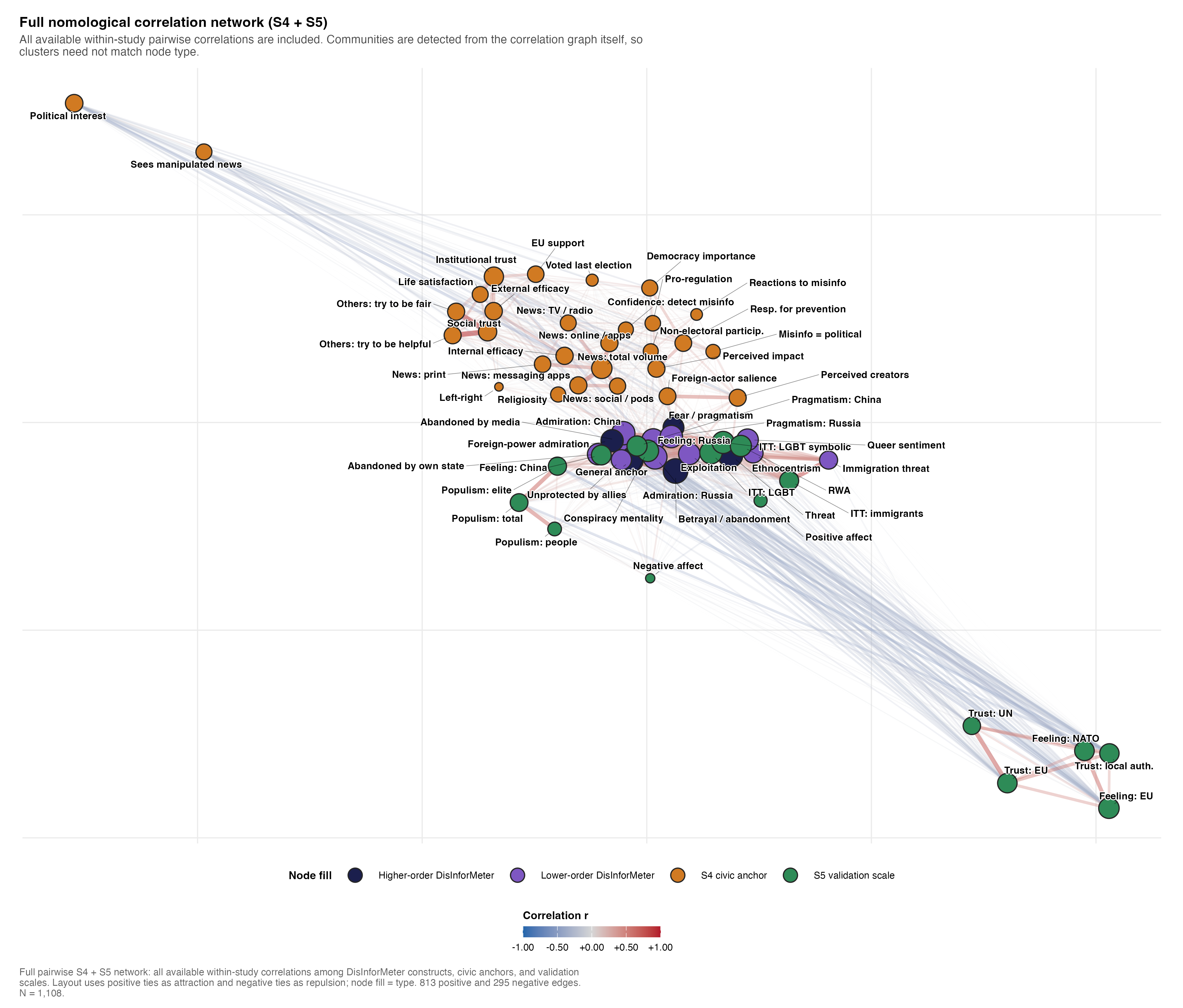
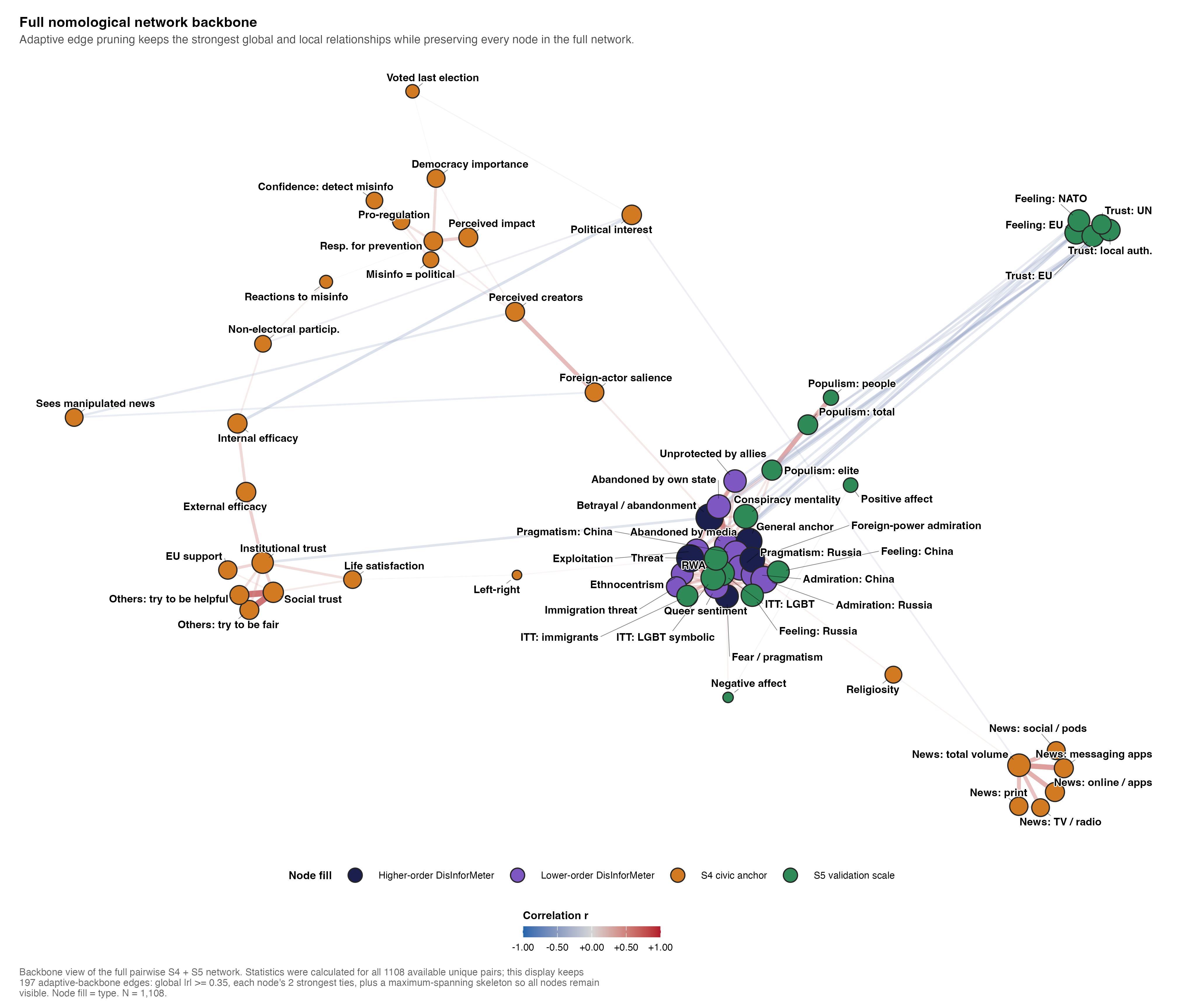
The network figures visualise the joined S4 + S5 correlation field between the DisInforMeter constructs and their nomological neighbours. They are interpretive layouts — the authoritative numeric correlations live in the anchor/validation tables above; the network shows the structure of those relationships.

Figure 11: Focal nomological network (force-directed). Edge colour = sign and strength of r (blue → red); node fill = node type.

Figure 12: Focal nomological network (radial / chord).

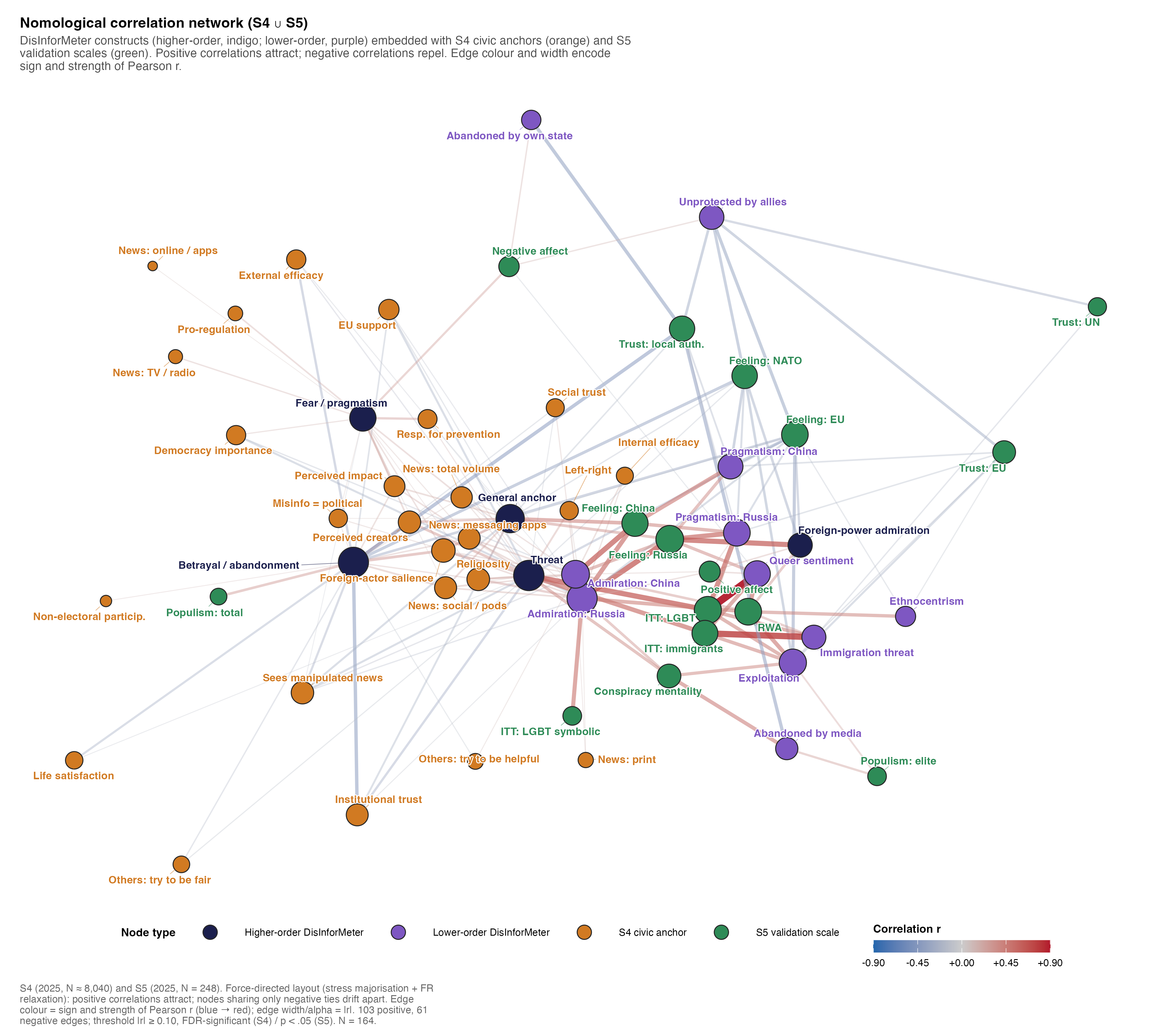
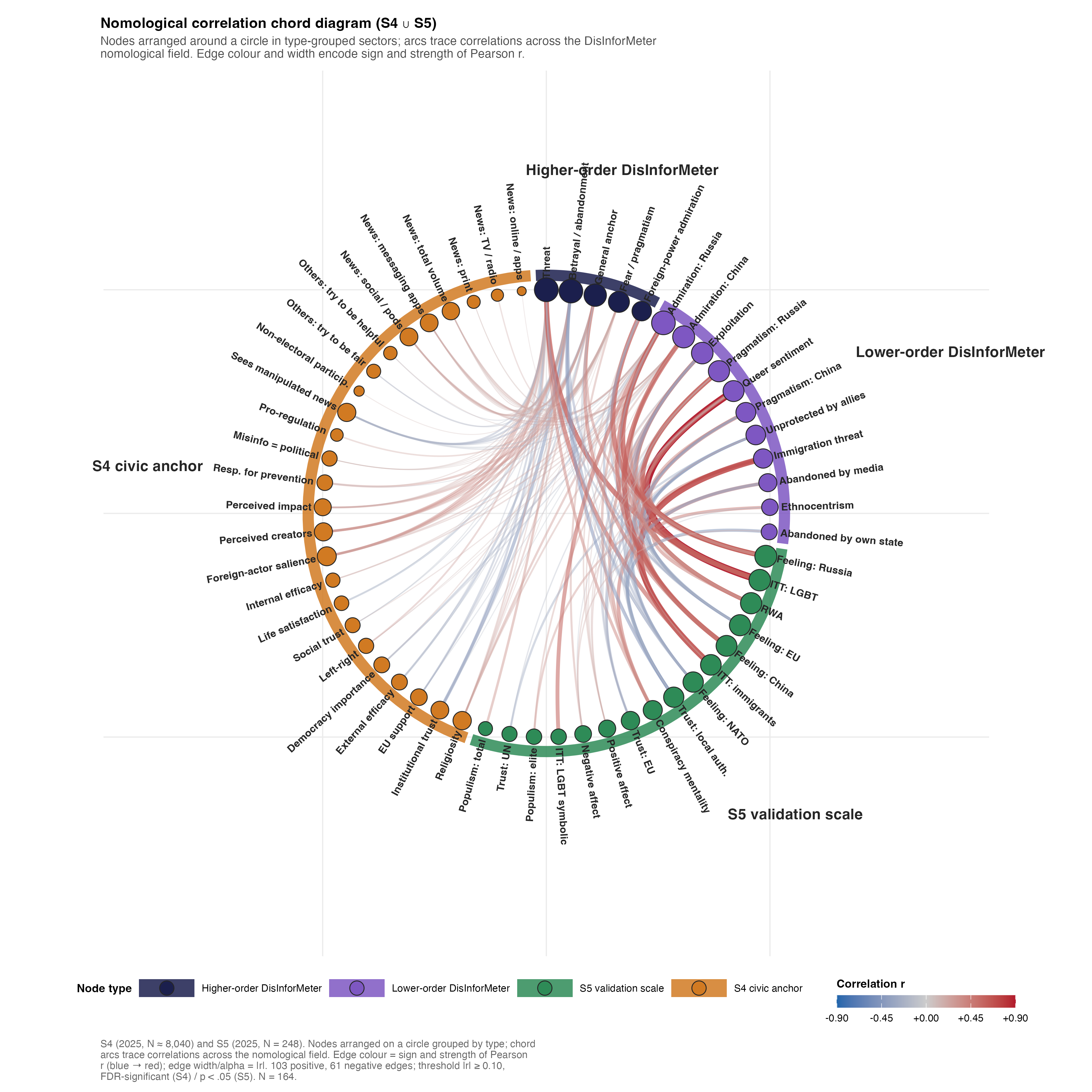
The full pairwise network (all aggregated within-study correlations across 62 nodes) is shown both in full and as an adaptive backbone that keeps every node on the canvas while reducing visual saturation.

Figure 13: Full pairwise network (force-directed): all 1,108 aggregated within-study correlations across 62 nodes.

Figure 14: Full network backbone: global |r| ≥ .35 plus each node’s two strongest ties plus a maximum-spanning skeleton (197 of 1,108 edges at the current cut).

R/policy_report/14_nomological_network.R (network edge/node producer)

#' R/policy_report/14_nomological_network.R
#'
#' Build a unified edge + node list from the S4 civic-anchor correlation
#' table and the S5 nomological-validation table. The output drives the
#' two correlation-network figures F-31 (force-directed) and F-32
#' (radial / chord).
#'
#' Inputs:
#'   outputs/tables/s4_external_anchor_correlations.csv  (S4: HO DisInforMeter
#'                                                         × 29 civic anchors)
#'   outputs/tables/s5_validation_results.csv            (S5: HO + LO
#'                                                         DisInforMeter × 13
#'                                                         validation scales)
#'
#' Outputs (under outputs/policy_report/cache/):
#'   nomological_network_edges.csv   long edge list
#'   nomological_network_nodes.csv   node table with type + label + family
#'
#' Edge schema
#' -----------
#'   from_id, to_id           canonical node ids on either side
#'   from_type, to_type       one of {ho_disinfo, lo_disinfo, civic_anchor,
#'                                    validation_scale}
#'   r                        correlation (S4: pooled r; S5: Pearson r)
#'   n                        sample size
#'   p                        two-sided p
#'   p_fdr                    FDR-corrected p (NA for S5; we only run FDR on
#'                            the larger S4 grid)
#'   source_study             "S4" or "S5"
#'   significant              TRUE iff p_fdr < .05 (S4) or p < .05 (S5)
#'   abs_r                    abs(r), used by ggraph for layout weight
#'   sign                     -1, 0, or +1
#'
#' Node schema
#' -----------
#'   id, label, short_label, type, family, source_study, n_edges
#'
#' Construct mapping is documented inline. Lower-order labels follow the S5
#' construct_label field; higher-order labels mirror those in
#' R/policy_report/_helpers.R::higher_order_construct_map().

source(here::here("R", "policy_report", "_helpers.R"))

suppressPackageStartupMessages({
  library(dplyr)
  library(tidyr)
  library(readr)
  library(tibble)
  library(stringr)
  library(purrr)
})

# ---------------------------------------------------------------------------
# Canonical mapping: S4 / S5 construct labels -> unified node ids + types
# ---------------------------------------------------------------------------

#' S4 predictor_label -> canonical id + type.
#' S4 carries six "higher-order" composites in the anchor table; SUPF /
#' SUPFCH are the foreign-power admiration anchors at the Russian and
#' Chinese facet level and are classified as lower-order in the unified
#' taxonomy (the higher-order roll-up SUP_GEN is provided by S5 only).
.s4_node_map <- function() {
  tibble::tribble(
    ~predictor_label, ~node_id,  ~node_type,    ~node_label,
    "GEN",            "GEN",     "ho_disinfo",  "General anchor",
    "THREAT",         "THREAT",  "ho_disinfo",  "Threat",
    "ABAND",          "ABAND",   "ho_disinfo",  "Betrayal / abandonment",
    "FEAR",           "FEAR",    "ho_disinfo",  "Fear / pragmatism",
    "SUPF",           "SUP_RU",  "lo_disinfo",  "Admiration: Russia",
    "SUPFCH",         "SUP_CH",  "lo_disinfo",  "Admiration: China"
  )
}

#' S5 construct_label -> canonical id + type.
#' Higher-order rows correspond to the "[general]" / "General" labels which
#' aggregate the S5-only facets; everything else is lower-order.
.s5_node_map <- function() {
  tibble::tribble(
    ~construct_label,                       ~node_id,      ~node_type,    ~node_label,
    # higher-order
    "General",                              "GEN",         "ho_disinfo",  "General anchor",
    "Threat [general]",                     "THREAT",      "ho_disinfo",  "Threat",
    "Abandoned [general]",                  "ABAND",       "ho_disinfo",  "Betrayal / abandonment",
    "Fear [general]",                       "FEAR",        "ho_disinfo",  "Fear / pragmatism",
    "Superiority [general]",                "SUP_GEN",     "ho_disinfo",  "Foreign-power admiration",
    # lower-order — Threat facets
    "Exploitation",                         "EXPL",        "lo_disinfo",  "Exploitation",
    "Queer Sentiment",                      "GAY",         "lo_disinfo",  "Queer sentiment",
    "Immigration",                          "MIGR",        "lo_disinfo",  "Immigration threat",
    "Poisonous ethnocentrism",              "CET",         "lo_disinfo",  "Ethnocentrism",
    # lower-order — Aband facets
    "Unprotected by international allies",  "UNP",         "lo_disinfo",  "Unprotected by allies",
    "Abandoned by media (censorship)",      "CEN",         "lo_disinfo",  "Abandoned by media",
    "Abandoned by own state",               "ABAN_STATE",  "lo_disinfo",  "Abandoned by own state",
    # lower-order — Fear facets
    "Pragmatism Russia",                    "PRAG_RU",     "lo_disinfo",  "Pragmatism: Russia",
    "Pragmatism China",                     "PRAG_CH",     "lo_disinfo",  "Pragmatism: China",
    # lower-order — Admiration facets
    "Superiority Russia",                   "SUP_RU",      "lo_disinfo",  "Admiration: Russia",
    "Superiority China",                    "SUP_CH",      "lo_disinfo",  "Admiration: China"
  )
}

# Civic anchors (S4) -- map family from anchor_corrs long table directly; we
# only need to assign short labels for readability. Anchor labels exceed 30
# chars in several cases.
.civic_anchor_short_labels <- c(
  "Democracy importance"                        = "Democracy importance",
  "EU support"                                  = "EU support",
  "External political efficacy"                 = "External efficacy",
  "Generalised social trust"                    = "Social trust",
  "Institutional trust"                         = "Institutional trust",
  "Internal political efficacy"                 = "Internal efficacy",
  "Left-right self-placement"                   = "Left-right",
  "Life satisfaction"                           = "Life satisfaction",
  "Political interest"                          = "Political interest",
  "Religiosity"                                 = "Religiosity",
  "Confidence detecting misinfo"                = "Confidence: detect misinfo",
  "Foreign-actor topic salience"                = "Foreign-actor salience",
  "Misinfo seen as political"                   = "Misinfo = political",
  "Perceived misinfo creators"                  = "Perceived creators",
  "Perceived misinfo impact"                    = "Perceived impact",
  "Pro-regulation of misinfo"                   = "Pro-regulation",
  "Responsibility for prevention"               = "Resp. for prevention",
  "Frequency of seeing manipulated news"        = "Sees manipulated news",
  "Non-electoral participation (count)"         = "Non-electoral particip.",
  "Reactions to suspected misinformation (count)" = "Reactions to misinfo",
  "Voted in last national election"             = "Voted last election",
  "Belief others try to be fair"                = "Others: try to be fair",
  "Belief others try to be helpful"             = "Others: try to be helpful",
  "News use — TV / radio"                       = "News: TV / radio",
  "News use — aggregate"                        = "News: total volume",
  "News use — messaging apps"                   = "News: messaging apps",
  "News use — online news / apps"               = "News: online / apps",
  "News use — print"                            = "News: print",
  "News use — social media / podcasts"          = "News: social / pods"
)

# S5 validation labels -> short labels (kept compact for ggraph node text).
.validation_short_labels <- c(
  "Conspiracy Mentality Questionnaire (CMQ; 5-item)"     = "Conspiracy mentality",
  "Populist attitudes scale (Silva, 2017)"               = "Populist attitudes",
  "Institutional trust battery (ESS) - EU"               = "Trust: EU",
  "Institutional trust battery (ESS) - United Nations"   = "Trust: UN",
  "Right Wing Authoritarianism (RWA short scale)"        = "RWA",
  "Intergroup threat scale (ITT) - LQBT"                 = "ITT: LGBT",
  "Intergroup threat scale (ITT) - Immigrants"           = "ITT: immigrants",
  "feeling thermometer - EU"                             = "Feeling: EU",
  "feeling thermometer - NATO"                           = "Feeling: NATO",
  "feeling thermometer - Russia"                         = "Feeling: Russia",
  "feeling thermometer - China"                          = "Feeling: China",
  "Institutional trust battery (ESS) - Local Authorities" = "Trust: local auth.",
  "Trait affectivity (I‑PANAS‑SF)"             = "Negative affect"
)

.label_from_col <- function(x) {
  x %>%
    stringr::str_remove("^scale_") %>%
    stringr::str_replace_all("_", " ") %>%
    stringr::str_to_sentence()
}

.validation_col_short_labels <- c(
  scale_cmq = "Conspiracy mentality",
  scale_pop = "Populism: total",
  scale_pop_people = "Populism: people",
  scale_pop_elite = "Populism: elite",
  scale_trust_local = "Trust: local auth.",
  scale_trust_eu = "Trust: EU",
  scale_trust_un = "Trust: UN",
  scale_feel_eu = "Feeling: EU",
  scale_feel_nato = "Feeling: NATO",
  scale_feel_ru = "Feeling: Russia",
  scale_feel_ch = "Feeling: China",
  scale_rwa = "RWA",
  scale_itt_imi = "ITT: immigrants",
  scale_itt_lgbt = "ITT: LGBT",
  scale_itt_lgbt_sym = "ITT: LGBT symbolic",
  scale_panas_pa = "Positive affect",
  scale_panas_na = "Negative affect"
)

.validation_short_label <- function(validation_col, validation_label) {
  by_col <- unname(.validation_col_short_labels[validation_col])
  by_label <- unname(.validation_short_labels[validation_label])
  dplyr::coalesce(by_col, by_label, .label_from_col(validation_col))
}

.s4_predictor_catalog <- function() {
  .s4_node_map() %>%
    dplyr::transmute(
      column = predictor_label,
      source_column = dplyr::case_when(
        predictor_label == "GEN"    ~ "scale_gen",
        predictor_label == "THREAT" ~ "scale_threat_long",
        predictor_label == "ABAND"  ~ "scale_aband_long",
        predictor_label == "FEAR"   ~ "scale_prag_long",
        predictor_label == "SUPF"   ~ "scale_supr",
        predictor_label == "SUPFCH" ~ "scale_supch",
        TRUE ~ NA_character_
      ),
      id = node_id,
      type = node_type,
      label = node_label,
      family = dplyr::if_else(type == "ho_disinfo",
                              "Higher-order DisInforMeter",
                              "Lower-order DisInforMeter")
    )
}

.s4_anchor_catalog <- function(anchor_tbl = NULL) {
  if (is.null(anchor_tbl)) {
    anchor_tbl <- readr::read_csv(policy_report_paths()$anchor_corrs,
                                  show_col_types = FALSE)
  }
  anchor_tbl %>%
    dplyr::distinct(anchor, anchor_label, family) %>%
    dplyr::transmute(
      source_column = anchor,
      id = paste0("ANCH_", toupper(stringr::str_replace_all(anchor, "[^A-Za-z0-9]+", "_"))),
      type = "civic_anchor",
      label = unname(.civic_anchor_short_labels[anchor_label]),
      family = family
    )
}

.s5_construct_catalog <- function() {
  tibble::tribble(
    ~construct_label,                       ~source_column,
    "General",                              "scale_gen",
    "Threat [general]",                     "scale_threat",
    "Abandoned [general]",                  "scale_aband",
    "Fear [general]",                       "scale_fear",
    "Superiority [general]",                "scale_sup_gen",
    "Exploitation",                         "scale_expl",
    "Queer Sentiment",                      "scale_gay",
    "Immigration",                          "scale_migr",
    "Poisonous ethnocentrism",              "scale_cet",
    "Unprotected by international allies",  "scale_unp",
    "Abandoned by media (censorship)",      "scale_cen",
    "Abandoned by own state",               "scale_aban_state",
    "Pragmatism Russia",                    "scale_pragr",
    "Pragmatism China",                     "scale_pragch",
    "Superiority Russia",                   "scale_supr",
    "Superiority China",                    "scale_supch"
  ) %>%
    dplyr::left_join(.s5_node_map(), by = "construct_label") %>%
    dplyr::transmute(
      source_column,
      id = node_id,
      type = node_type,
      label = node_label,
      family = dplyr::if_else(type == "ho_disinfo",
                              "Higher-order DisInforMeter",
                              "Lower-order DisInforMeter")
    )
}

.s5_validation_catalog <- function(results = NULL) {
  if (is.null(results)) {
    results <- readr::read_csv(here::here("outputs", "tables",
                                          "s5_validation_results.csv"),
                               show_col_types = FALSE)
  }
  results %>%
    dplyr::filter(is.na(item_subset_label), is.na(skip_reason)) %>%
    dplyr::distinct(validation_col, validation_label) %>%
    dplyr::transmute(
      source_column = validation_col,
      id = paste0("VAL_", toupper(stringr::str_replace_all(validation_col, "[^A-Za-z0-9]+", "_"))),
      type = "validation_scale",
      label = .validation_short_label(validation_col, validation_label),
      family = "Validation scale"
    )
}

.s4_full_frame <- function() {
  paths <- policy_report_paths()
  s4_scales <- arrow::read_parquet(paths$s4_scales)
  s4_items  <- arrow::read_parquet(paths$s4_items)

  s4_scales %>%
    dplyr::left_join(
      s4_items %>%
        dplyr::transmute(
          response_id,
          anchor_voted = dplyr::case_when(
            q24 == 1 ~ 1,
            q24 == 2 ~ 0,
            TRUE ~ NA_real_
          ),
          anchor_news_manip_freq = q9,
          anchor_fair_belief = q18,
          anchor_helpful_belief = q19,
          anchor_media_print = q3_1,
          anchor_media_tv_radio = q3_2,
          anchor_media_online = q3_3,
          anchor_media_messaging = q3_4,
          anchor_media_social = q3_5
        ),
      by = "response_id"
    )
}

.pairwise_cor_edges <- function(df, nodes, source_study) {
  nodes <- nodes %>%
    dplyr::filter(source_column %in% names(df)) %>%
    dplyr::distinct(id, source_column, .keep_all = TRUE)
  if (nrow(nodes) < 2L) {
    return(tibble::tibble())
  }

  pairs <- utils::combn(nodes$source_column, 2, simplify = FALSE)
  purrr::map_dfr(pairs, function(pair) {
    a <- nodes %>% dplyr::filter(source_column == pair[[1]]) %>% dplyr::slice(1)
    b <- nodes %>% dplyr::filter(source_column == pair[[2]]) %>% dplyr::slice(1)
    cc <- stats::complete.cases(df[, pair, drop = FALSE])
    n <- sum(cc)
    if (n < 10L ||
        stats::sd(df[[pair[[1]]]][cc], na.rm = TRUE) == 0 ||
        stats::sd(df[[pair[[2]]]][cc], na.rm = TRUE) == 0) {
      r <- NA_real_; p <- NA_real_
    } else {
      ct <- suppressWarnings(stats::cor.test(df[[pair[[1]]]][cc],
                                             df[[pair[[2]]]][cc]))
      r <- unname(ct$estimate)
      p <- ct$p.value
    }
    tibble::tibble(
      from_id = a$id,
      to_id = b$id,
      from_type = a$type,
      to_type = b$type,
      from_label = a$label,
      to_label = b$label,
      from_family = a$family,
      to_family = b$family,
      r = r,
      n = n,
      p = p,
      source_study = source_study,
      edge_scope = dplyr::case_when(
        stringr::str_detect(a$type, "disinfo") & stringr::str_detect(b$type, "disinfo") ~ "within_disinformeter",
        !stringr::str_detect(a$type, "disinfo") & !stringr::str_detect(b$type, "disinfo") ~ "within_external",
        TRUE ~ "cross_domain"
      )
    )
  }) %>%
    dplyr::filter(!is.na(r))
}

.fisher_average <- function(r, n) {
  ok <- !is.na(r) & !is.na(n) & n > 3
  if (!any(ok)) return(NA_real_)
  r <- pmin(pmax(r[ok], -0.999999), 0.999999)
  w <- pmax(n[ok] - 3, 1)
  tanh(stats::weighted.mean(atanh(r), w = w))
}

.aggregate_full_edges <- function(edges) {
  edges %>%
    dplyr::mutate(
      id_a = pmin(from_id, to_id),
      id_b = pmax(from_id, to_id)
    ) %>%
    dplyr::group_by(id_a, id_b) %>%
    dplyr::summarise(
      r = .fisher_average(r, n),
      n = max(n, na.rm = TRUE),
      p = if (dplyr::n() == 1L) dplyr::first(p) else NA_real_,
      source_study = paste(sort(unique(source_study)), collapse = " + "),
      source_edge_count = dplyr::n(),
      edge_scope = paste(sort(unique(edge_scope)), collapse = " + "),
      .groups = "drop"
    ) %>%
    dplyr::transmute(
      from_id = id_a,
      to_id = id_b,
      r,
      n,
      p,
      p_fdr = stats::p.adjust(p, method = "BH"),
      source_study,
      source_edge_count,
      edge_scope,
      significant = dplyr::if_else(is.na(p), NA, p < 0.05),
      abs_r = abs(r),
      sign = sign(r)
    )
}

# ---------------------------------------------------------------------------
# Edge builders
# ---------------------------------------------------------------------------

#' Build the S4 (HO DisInforMeter × civic anchor) edges.
#'
#' Keeps edges where |r| >= `min_r` and `p_fdr < .05`. Default threshold is
#' 0.10 because the S4 N is ~8,000 — at that N a |r| of 0.03 is still
#' "significant" but not meaningful.
.build_s4_edges <- function(min_r = 0.10) {
  paths <- policy_report_paths()
  long  <- readr::read_csv(paths$anchor_corrs, show_col_types = FALSE)

  s4_map <- .s4_node_map()
  long %>%
    dplyr::transmute(
      from_id      = s4_map$node_id[match(predictor_label, s4_map$predictor_label)],
      from_type    = s4_map$node_type[match(predictor_label, s4_map$predictor_label)],
      from_label   = s4_map$node_label[match(predictor_label, s4_map$predictor_label)],
      to_label_long = anchor_label,
      to_label     = unname(.civic_anchor_short_labels[anchor_label]),
      to_id        = paste0("ANCH_", toupper(stringr::str_replace_all(anchor, "[^A-Za-z0-9]+", "_"))),
      to_type      = "civic_anchor",
      family       = family,
      r            = r_pooled,
      n            = n_pooled,
      p            = p_pooled,
      p_fdr        = p_fdr,
      source_study = "S4",
      significant  = !is.na(p_fdr) & p_fdr < 0.05
    ) %>%
    dplyr::filter(!is.na(r), significant, abs(r) >= min_r)
}

#' Build the S5 (HO + LO DisInforMeter × validation scale) edges.
#'
#' Filters: primary-row only (`is.na(item_subset_label)`), no skip reason,
#' `|r| >= min_r`. We use Pearson r as the canonical correlation; Spearman
#' is available but the S4 side is Pearson so this keeps the two studies
#' comparable.
.build_s5_edges <- function(min_r = 0.10) {
  raw <- readr::read_csv(here::here("outputs", "tables",
                                     "s5_validation_results.csv"),
                          show_col_types = FALSE)

  s5_map <- .s5_node_map()
  raw %>%
    dplyr::filter(is.na(item_subset_label),
                  is.na(skip_reason),
                  !is.na(r)) %>%
    dplyr::transmute(
      from_id      = s5_map$node_id[match(construct_label, s5_map$construct_label)],
      from_type    = s5_map$node_type[match(construct_label, s5_map$construct_label)],
      from_label   = s5_map$node_label[match(construct_label, s5_map$construct_label)],
      to_label_long = validation_label,
      to_label     = .validation_short_label(validation_col, validation_label),
      to_id        = paste0("VAL_", toupper(stringr::str_replace_all(validation_col, "[^A-Za-z0-9]+", "_"))),
      to_type      = "validation_scale",
      family       = "Validation scale",
      r            = r,
      n            = n,
      p            = p_two_sided,
      p_fdr        = NA_real_,
      source_study = "S5",
      significant  = !is.na(p_two_sided) & p_two_sided < 0.05
    ) %>%
    dplyr::filter(abs(r) >= min_r, significant)
}

# ---------------------------------------------------------------------------
# Compute + main
# ---------------------------------------------------------------------------

compute_nomological_network <- function(min_r = 0.10) {
  edges_s4 <- .build_s4_edges(min_r = min_r)
  edges_s5 <- .build_s5_edges(min_r = min_r)

  if (anyNA(edges_s4$from_id))
    stop("[14] Unmapped S4 predictor_label -- update .s4_node_map().",
         call. = FALSE)
  if (anyNA(edges_s5$from_id))
    stop("[14] Unmapped S5 construct_label -- update .s5_node_map().",
         call. = FALSE)
  if (anyNA(edges_s4$to_label))
    stop("[14] Unmapped S4 civic anchor -- update .civic_anchor_short_labels.",
         call. = FALSE)
  if (anyNA(edges_s5$to_label))
    stop("[14] Unmapped S5 validation_label -- update .validation_short_labels.",
         call. = FALSE)

  edges <- dplyr::bind_rows(edges_s4, edges_s5) %>%
    dplyr::mutate(
      abs_r = abs(r),
      sign  = sign(r)
    )

  # Build the node table.
  from_nodes <- edges %>%
    dplyr::distinct(id = from_id, type = from_type, label = from_label) %>%
    dplyr::mutate(family = dplyr::if_else(type == "ho_disinfo",
                                           "Higher-order DisInforMeter",
                                           "Lower-order DisInforMeter"))

  to_nodes <- edges %>%
    dplyr::distinct(id = to_id, type = to_type, label = to_label,
                    family = family)

  nodes <- dplyr::bind_rows(from_nodes, to_nodes) %>%
    dplyr::distinct(id, type, .keep_all = TRUE)

  # n_edges per node (used by F-31 for sizing).
  deg <- edges %>%
    dplyr::select(from_id, to_id, abs_r) %>%
    tidyr::pivot_longer(c(from_id, to_id), values_to = "id") %>%
    dplyr::group_by(id) %>%
    dplyr::summarise(
      n_edges = dplyr::n(),
      sum_abs_r = sum(abs_r, na.rm = TRUE),
      .groups   = "drop"
    )

  nodes <- nodes %>%
    dplyr::left_join(deg, by = "id") %>%
    dplyr::mutate(n_edges   = tidyr::replace_na(n_edges, 0L),
                  sum_abs_r = tidyr::replace_na(sum_abs_r, 0))

  list(edges = edges, nodes = nodes)
}

compute_nomological_full_network <- function() {
  anchor_tbl <- readr::read_csv(policy_report_paths()$anchor_corrs,
                                show_col_types = FALSE)
  s5_results <- readr::read_csv(here::here("outputs", "tables",
                                           "s5_validation_results.csv"),
                                show_col_types = FALSE)

  s4_nodes <- dplyr::bind_rows(
    .s4_predictor_catalog(),
    .s4_anchor_catalog(anchor_tbl)
  ) %>%
    dplyr::filter(!is.na(id), !is.na(label))

  s5_nodes <- dplyr::bind_rows(
    .s5_construct_catalog(),
    .s5_validation_catalog(s5_results)
  ) %>%
    dplyr::filter(!is.na(id), !is.na(label))

  s4_edges_raw <- .pairwise_cor_edges(.s4_full_frame(), s4_nodes, "S4")
  s5_edges_raw <- .pairwise_cor_edges(arrow::read_parquet(policy_report_paths()$s5_scales),
                                      s5_nodes, "S5")

  raw_edges <- dplyr::bind_rows(s4_edges_raw, s5_edges_raw)
  edges <- .aggregate_full_edges(raw_edges)

  node_lookup <- dplyr::bind_rows(
    s4_nodes %>% dplyr::select(id, type, label, family),
    s5_nodes %>% dplyr::select(id, type, label, family)
  ) %>%
    dplyr::distinct(id, .keep_all = TRUE)

  nodes_used <- tibble::tibble(id = unique(c(edges$from_id, edges$to_id))) %>%
    dplyr::left_join(node_lookup, by = "id")

  if (anyNA(nodes_used$type) || anyNA(nodes_used$label)) {
    missing_ids <- nodes_used$id[is.na(nodes_used$type) | is.na(nodes_used$label)]
    stop("[14] Full network has unmapped node ids: ",
         paste(missing_ids, collapse = ", "), call. = FALSE)
  }

  deg <- edges %>%
    dplyr::select(from_id, to_id, abs_r) %>%
    tidyr::pivot_longer(c(from_id, to_id), values_to = "id") %>%
    dplyr::group_by(id) %>%
    dplyr::summarise(
      n_edges = dplyr::n(),
      sum_abs_r = sum(abs_r, na.rm = TRUE),
      .groups = "drop"
    )

  nodes <- nodes_used %>%
    dplyr::left_join(deg, by = "id") %>%
    dplyr::mutate(
      n_edges = tidyr::replace_na(n_edges, 0L),
      sum_abs_r = tidyr::replace_na(sum_abs_r, 0)
    )

  list(edges = edges, nodes = nodes, raw_edges = raw_edges)
}

main_14 <- function() {
  paths <- policy_report_paths()
  ensure_policy_report_dirs()

  res <- compute_nomological_network()
  edges <- res$edges; nodes <- res$nodes
  full_res <- compute_nomological_full_network()
  full_edges <- full_res$edges
  full_nodes <- full_res$nodes
  full_raw_edges <- full_res$raw_edges

  validate_policy_report_table(
    edges,
    label = "14 / nomological_network_edges.csv",
    required_cols = c("from_id", "to_id", "from_type", "to_type",
                      "r", "abs_r", "sign", "source_study"),
    country_col = NULL,
    range_checks = list(r = c(-1, 1), abs_r = c(0, 1))
  )

  validate_policy_report_table(
    nodes,
    label = "14 / nomological_network_nodes.csv",
    required_cols = c("id", "type", "label", "family", "n_edges"),
    country_col = NULL
  )

  validate_policy_report_table(
    full_edges,
    label = "14 / nomological_network_full_edges.csv",
    required_cols = c("from_id", "to_id", "r", "abs_r", "sign",
                      "source_study", "edge_scope"),
    country_col = NULL,
    range_checks = list(r = c(-1, 1), abs_r = c(0, 1))
  )

  validate_policy_report_table(
    full_nodes,
    label = "14 / nomological_network_full_nodes.csv",
    required_cols = c("id", "type", "label", "family", "n_edges"),
    country_col = NULL
  )

  policy_report_message(sprintf("  edges: %d (S4: %d, S5: %d)",
                                nrow(edges),
                                sum(edges$source_study == "S4"),
                                sum(edges$source_study == "S5")))
  policy_report_message(sprintf("  nodes: %d (%s)",
                                nrow(nodes),
                                paste(sort(unique(nodes$type)), collapse = ", ")))
  policy_report_message(sprintf("  |r| range: [%.2f, %.2f]",
                                min(edges$abs_r), max(edges$abs_r)))
  policy_report_message(sprintf("  full pairwise edges: %d raw -> %d aggregated",
                                nrow(full_raw_edges), nrow(full_edges)))
  policy_report_message(sprintf("  full pairwise nodes: %d (%s)",
                                nrow(full_nodes),
                                paste(sort(unique(full_nodes$type)), collapse = ", ")))
  policy_report_message(sprintf("  full |r| range: [%.2f, %.2f]",
                                min(full_edges$abs_r), max(full_edges$abs_r)))

  out_edges <- file.path(paths$cache, "nomological_network_edges.csv")
  out_nodes <- file.path(paths$cache, "nomological_network_nodes.csv")
  out_full_edges <- file.path(paths$cache, "nomological_network_full_edges.csv")
  out_full_nodes <- file.path(paths$cache, "nomological_network_full_nodes.csv")
  out_full_raw <- file.path(paths$cache, "nomological_network_full_source_edges.csv")
  readr::write_csv(edges, out_edges)
  readr::write_csv(nodes, out_nodes)
  readr::write_csv(full_edges, out_full_edges)
  readr::write_csv(full_nodes, out_full_nodes)
  readr::write_csv(full_raw_edges, out_full_raw)
  policy_report_message(sprintf("wrote %s", out_edges))
  policy_report_message(sprintf("wrote %s", out_nodes))
  policy_report_message(sprintf("wrote %s", out_full_edges))
  policy_report_message(sprintf("wrote %s", out_full_nodes))
  policy_report_message(sprintf("wrote %s", out_full_raw))

  invisible(list(thresholded = res, full = full_res))
}

if (sys.nframe() == 0L) main_14()

Downloads: s4_country_predictor_paths_brms_full.csv · s4_country_predictor_paths_brms_russian.csv · s4_country_predictor_paths_brms_chinese.csv · s4_anchor_correlations_wide.csv

References

Akkerman, A., Mudde, C., & Zaslove, A. (2014). How populist are the people? Measuring populist attitudes in voters. Comparative Political Studies, 47(9), 1324–1353. https://doi.org/10.1177/0010414013512600

Bruder, M., Haffke, P., Neave, N., Nouripanah, N., & Imhoff, R. (2013). Measuring individual differences in generic beliefs in conspiracy theories across cultures: The conspiracy mentality questionnaire. Frontiers in Psychology, 4, 225. https://doi.org/10.3389/fpsyg.2013.00225

Campbell, D. T., & Fiske, D. W. (1959). Convergent and discriminant validation by the multitrait-multimethod matrix. Psychological Bulletin, 56(2), 81–105. https://doi.org/10.1037/h0046016

ESS. (2024). ESS round 11 source questionnaire. European Social Survey ERIC. https://www.europeansocialsurvey.org/news/article/round-11-questionnaire-and-provisional-release-dates

Niemi, R. G., Craig, S. C., & Mattei, F. (1991). Measuring internal political efficacy in the 1988 national election study. American Political Science Review, 85(4), 1407–1413. https://doi.org/10.2307/1963953

OECD. (2017). OECD guidelines on measuring trust. OECD Publishing. https://doi.org/10.1787/9789264278219-en

Shadish, W. R., Cook, T. D., & Campbell, D. T. (2002). Experimental and quasi-experimental designs for generalized causal inference. Houghton Mifflin.

Stephan, W. G., Ybarra, O., & Morrison, K. R. (2009). Intergroup threat theory. In T. D. Nelson (Ed.), Handbook of prejudice, stereotyping, and discrimination (pp. 43–59). Psychology Press.